We're going to calculate a value for π by numerical integration. To do this we're going to calculate the area of a quadrant of a circle. The ancient Greeks called finding the area "squaring", as their method used geometric transformations of the object into squares, for which they knew the area. The Greeks knew how to square a rectangle, triangle (and hence a parallelogram). They did not know how to square a circle (the problem being that π is irrational). In modern time (1500's or so), people found ways of squaring the area under parabolas (and other polynomial curves), but had difficulty with squaring the area under a hyperbola. All these problems were swept away by the invention of calculus by Newton and Leibnitz. Calculus cut areas into infinitesimal slices and summed them. This was not as rigorous as the Greek method, but gave useful (and correct) answers. People now accept that the Greek method could not be extended further and that the methods of calculus are acceptable. Since the Greek methods don't work for most problems, the term "squaring" has been replaced with "finding the area".
numerical: we're going to cut a quarter circle into rectangular strips and measure the area of each strip (ignoring that one end of the strip is part of the arc of a circle, rather than a straight line). It's numerical because we're not going to derive a formula for π - we're going to calculate the value by brute force summing of areas (this is what computers do well).
integration: if we integrate a line (e.g. a quarter circle), this means that we calculate the area under the line. If we integrate the plot (graph) of a car's speed as a function of time, we'll get the distance the car travels. If we integrate under a surface (e.g. a hemisphere) we get the volume under the surface.
Some interesting info on π
- "The History of Pi", Petr Beckmann (available in at least two editions, 1971 Golem Press, 1993 Barnes and Noble). One of my favourite books.
- values of π through history (http://mathforum.org/isaac/problems/pi2.html).
- Ludolph van Ceulen and Pi (http://mathforum.org/library/drmath/view/52555.html)
Let's look at the part of the circle in the first quadrant. This diagram shows details for the point (x,y)=(0.6,0.8).
 | Note |
|---|---|
| The python code for the diagrams used in this section is here [159] . Since this code will only be run once, there's no attempt to make it fast. | |
Figure 4. Pythagorean formula for circumference of a circle
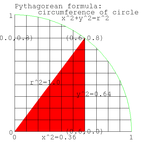 |
Pythagorean formula for circumference of a circle
From Pythagorus' theorem, we know that the distance from the center at (0,0), to any point (x,y) on the circumference of a circle of radius=1, is 1. The square of the distance to the center of the circle (the hypoteneus) is equal to the sum of the squares of the two sides, the lengths of which are given by (x,y). Thus we know that the locus of the circumference of a circle of radius 1 is
x*x + y*y = 1*1 |
| Note | ||||
|---|---|---|---|---|---|
locus: the path traced out by a point moving according to a law. Here's some examples. The circumference of a circle is the locus of a point which moves at constant distance from the center. A straight line is the locus of a point that moves along the path, which is the shortest distance between two points. An ellipse is the locus of a point which moves so that the sum of the distances to two points (the two focii) is constant. (The planets move around the sun in paths which are ellipses. The sun is one of the focii.)
| |||||
In the diagram above if x=0.6, then y=0.8. Let's confirm Pythagorus.
x^2=0.36, y^2=0.64; x^2+y^2=1. |
Rearranging the formula for the (locus of the) circumference, gives y (the height or ordinate) for any x (the abscissa).
x^2 + y^2 = 1^2 y^2 = 1-x^2 y = sqrt(1-x*x) |
i.e. for any x on the circumference, we can calculate y. e.g. x=0.6: what is y?
y = sqrt(1-x*x) = sqrt(1-0.36) = sqrt(0.64) = 0.8 |
If x=0.707, what is y [160] .
The point on the circle with y=0.5: what angle (by eyeball, or by marking off lengths around the circumference) does the line joining this point to the center, make with the x axis [161] .
Similarly we can calculate x knowing y.
x = sqrt(1-y*y) |
The value of π is known to many more decimal places than we can ever use on a 32 bit computer, so there's no need to calculate it again. Instead let's assume that either we don't know its value, or that we want to do the numerical integration on a problem whose answer is known, to check that we understand numerical integration.
The area of a circle is A=pi*r2, giving the area of the quadrant as pi/4. Knowing the locus of the circumference (we have a formula that gives y for any x), we will numerically calculate the area of the circle, thus giving us an estimate of the value of π.
If we divide the x axis into say 10 intervals, we can make these intervals the base of columns, whose tops intersect the highest part of the circle in that slice (which is on the left side of each slice).
Figure 5. Upper Bound of area under slices of a circle
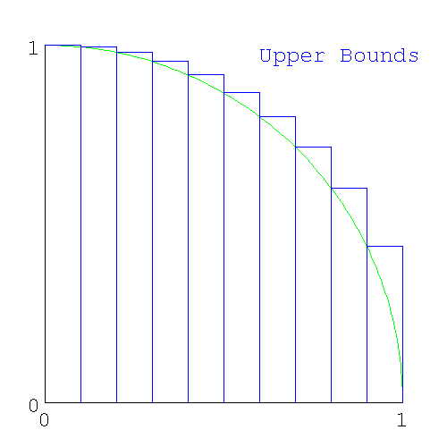 |
Upper Bound of area under slices of a circle
When we add these slices together, we'll get an area that is greater than π; i.e. we will have calculated an upper bound for π.
Here's the set of columns that intersect the lowest part of the circle in each interval (here the lowest part of the circle is on the right side of the slice).
Figure 6. Lower Bounds of area under slices of a circle
 |
Lower Bounds of area under slices of a circle
We can calculate the area of the two sets of columns. If we sum the sets of upper bound columns, we'll get an estimate which is guaranteed to be more than pi/4 and for the set of lower bound colums, a number guaranteed to be less than pi/4.
| Note |
|---|---|
We could have picked the point in the middle of the interval to calculate the area. The answer will be more accurate, but now we don't know how accurate (we don't even know if it's more or less than π). The advantage of the method used here is that we have an upper and lower bound for π, and so we know that the value of π is in this range. We could have used tighter bounds - lower bound by constructing a straight line joining the left and right end of each interval (giving a trapezoid), - upper bound by making a line tangent to the circle. (This is more bother than it's worth, and are left as an exercise for the student.) | |
If we progressively decrease the size of the interval (by changing from 10 intervals, to 100 intervals, to 1000 intervals..) the approximation to a circle by the columns will get better and better giving us progressively better estimates of pi/4. Here's the diagram with 100 slices.
Figure 7. Lower Bounds of area under 100 slices of a circle
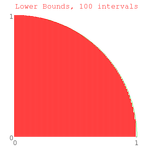 |
Lower Bounds of area under 100 slices of a circle
We have a problem similar to the fencepost error problem: how many heights do we need to calculate if we want to calculate both the upper and lower bounds for 10 intervals. [162] ?
Here's code to generate the heights of the required number of columns (you'll need sqrt(), from the math module). I ran this code in immediate mode, but you can write a file called slice_heights.py if you like.
>>> from math import sqrt >>> for x in range(0,11): ... print x, sqrt(1-1.0*x*x/100) ... 0 1.0 1 0.994987437107 2 0.979795897113 3 0.953939201417 4 0.916515138991 5 0.866025403784 6 0.8 7 0.714142842854 8 0.6 9 0.435889894354 10 0.0 |
Why did I use 11 as the 2nd argument to range() [163] ? What is the "1.0" doing in "1.0*x*x" [164] ?
| Note |
|---|---|
| End Lesson 24 | |
| Note | ||
|---|---|---|---|
Python is a scripting language, rather than a general purpose language. Python can only use integers for loop variables. To feed real values to a loop, python requires a construct like
where x,num_intervals make the real real_number. It's not immediately obvious that the calculations are ranging over values 0.0..1.0 (or more likely start..end). In most languages, real numbers can be used as loop variables, and can use the construct
Here it's clear that x is a real in the range start..end. | |||
Write code pi_lower.py to calculate the lower bound for π using 10 intervals. Use variable names num_intervals, height, area for the number of intervals, height of each column, and for the cumulative area. Start with a loop just calculating the height of each slice, printing the loop index and the height each time. For the print statement use something like
I've been using the single letter variable 'x' as the loop parameter thus far, since it's the loop parameter conveying the position on the x-axis. However loop parameters (in python) are integers, while the x position is a real (from 0.0..1.0). Usually loop parameters (which are integers) are just counters and are given simple variable names 'i,j,k,l...', which are easy to spot in code as they are so short. In this case the loop parameter is the number of the interval (which goes from 0..num_intervals). I tried writing the code with the name "interval" mixed in with "num_intervals" and it was hard to read. Instead I will use 'i'.
print "%d, %3.5f" %(x, height) |
When that's working, calculate the area of each slice and add it to the variable area. The area of each rectangle is height*base. You've just calculated height; what is the width of the base in terms of variables already in the code [165] ?
At the end, print out the lower bound for π with a line like
print "lower bound of pi %3.5f" %(area*4) |
Here's my code for pi_lower.py [166] and here's my output.
0, 0.99499, 0.09950 1, 0.97980, 0.19748 2, 0.95394, 0.29287 3, 0.91652, 0.38452 4, 0.86603, 0.47113 5, 0.80000, 0.55113 6, 0.71414, 0.62254 7, 0.60000, 0.68254 8, 0.43589, 0.72613 9, 0.00000, 0.72613 lower bound of pi 2.90452 |
Do the same for the upper bound of π writing a file pi_upper.py and using variables num_intervals, Height, Area (note variable names for the upper bounds start with uppercase, to differentiate them from the lower bounds variables). Here's my code [167] and here's my output.
0, 1.00000, 0.10000 1, 0.99499, 0.19950 2, 0.97980, 0.29748 3, 0.95394, 0.39287 4, 0.91652, 0.48452 5, 0.86603, 0.57113 6, 0.80000, 0.65113 7, 0.71414, 0.72254 8, 0.60000, 0.78254 9, 0.43589, 0.82613 upper bound for pi 3.30452 |
The two bounds (upper and lower, from the output of the two programs) show 2.9<pi<3.3 which agrees with the known value of π.
The two pieces of code look quite similar. Also note some of the numbers in the outputs are the same (how many are the same [168] ?) We should check for code duplication (in case we only need one piece of code).
Figure 8. Upper and Lower Bounds of area under a circle
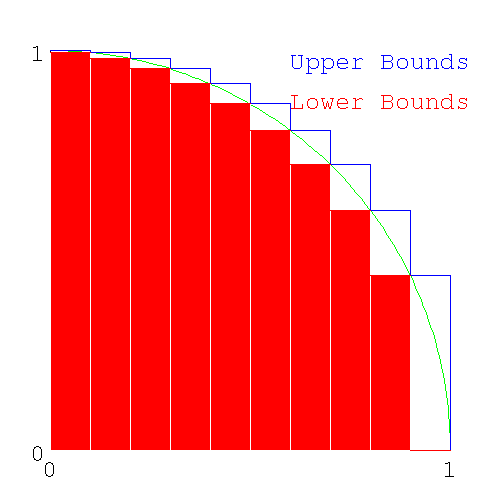 |
Upper and Lower Bounds of area under a circle
Looking at the diagram above which shows upper and lower bounds together, we see the following
- The height of the lower bound in one slice is the same as the upper bound for the next slice to the right.
- The difference between the upper and lower bounds (the series of white rectangles with the arc of the circumference going from the bottom right corner to the upper left corner), when added together, is the same as the height of the left most slice.
Redrawing the diagram, shifting the lower bounds slices one interval to the right shows
Figure 9. Upper and shifted Lower Bounds of area under a circle
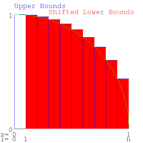 |
Upper and shifted Lower Bounds of area under a circle
This shows that the upper and lower bounds only differ by the area of the left most slice. This means only one loop of code is needed to calculate both bounds. Look in the output of pi_lower.py and pi_upper.py for the 9 numbers in common.
The duplication arises because the lower bound for one interval is the upper bound for the next interval and we only need to calculate it once. The first interval for the upper bound and the last interval for the lower bound are unique to each bound and will have to be calculated separately.
| Note |
|---|---|
| This is a general phenomenon: When calculating a value by determining an upper and lower bound, if the curve is monotonic, you should expect to find values that are used for both the upper and lower bound. | |
Write code (call the file pi_2.py - there is no pi.py anymore) to calculate the area common to both bounds (i.e. except for the two end pieces) in one loop. Use x for the loop control variable (the slice number), h for the height of each slice and a to accumulate the common area. In the loop output the variables for each iteration with a line like
print "%10d %10.20f %10.20f" %(x, h, a) |
After exiting the loop, add the two end areas, one for the lower bound and one for the upper bound to give area and Area and output your estimates of the lower and upper bounds for π with a line like
print "pi upper bound %10.20f, lower bound %10.20f" %(Area*4, area*4) |
Here's the code [169] and here's the output
pip:# ./pi_2.py 1 0.99498743710661996520 0.09949874371066200207 2 0.97979589711327119694 0.19747833342198911621 3 0.95393920141694565906 0.29287225356368368212 4 0.91651513899116798800 0.38452376746280048092 5 0.86602540378443859659 0.47112630784124431838 6 0.80000000000000004441 0.55112630784124427841 7 0.71414284285428497601 0.62254059212667278711 8 0.59999999999999997780 0.68254059212667272938 9 0.43588989435406727546 0.72612958156207940696 pi upper bound 3.304518, lower bound 2.904518 |
giving the same result: 2.9 < pi < 3.3
To get a more accurate result, we now increase the number of intervals, thus making the slices smaller and reducing the jaggyness of the approximation to the circle.
| Note |
|---|---|
| End Lesson 25 | |
| Note | ||||
|---|---|---|---|---|---|
Engineers take pride in being able to do what is called a back of the envelope calculation. While it may take weeks of computer time to get an accurate answer, an engineer should be able to get an approximate answer using only the back of an envelope to do the calculation (extra points are added if you can do it in the elevator between floors). As part of the calculation, you also need to be able determine the accuracy of your answer (is it correct within a factor of 100,10,2, 10%?) or state whether it's an upper or lower bound. If the answer is within reasonable bounds, then it's worth spending a few months and a lot of money to find the real answer. e.g. how long does it take to get from Earth to Mars using the minimum amount of fuel. It's going to be somewhere between the half the time of Earth's orbit and half the time of Mar's orbit (both planets orbit using no fuel at all), i.e. between 6 months and a year - let's make it 9 months. The answer is 8.6 months (Earth-Mars Hohmann trajectory http://www.newmars.com/wiki/index.php/Hohmann_trajectory).
| |||||
Before we change the number of intervals to some large number (like 109), we need some idea of the time this will take. We could change intervals to 10,100... and measure the time for the runs (the quite valid experimental approach) and extrapolate to 109 intervals. Another approach is to do a back of the envelope calculation of the amount of time we'll need. We don't need it to be accurate - we just need to know whether the run will take a second, an hour or a year, to see if it's feasible to run the code with intervals=109. Lets say we use 1G intervals. The calculation goes like this
- our computer has a clock rate of 1GHz, meaning that it can do 1G operations/sec (approximately).
- the for loop is executed once for each interval. Let's say there are 100 operations/loop (rough guess, we could be out by a factor of 10, but that's close enough for the moment)
A 1GHz computer then will take about 100 secs for num_intervals=109. If you have a 128MHz computer, expect the run to be 8 times longer (800secs=13mins). In this case, you may not be able to do a run with num_intervals=109 in class time, but you should be able to do a run with num_intervals=108.
Do multiple runs of pi_2.py increasing num_intervals by a factor of 10-100 each time, noticing the changes in the upper and lower bounds for π. (Comment out the print() statement inside the loop or it will take forever.)
| Note |
|---|---|
| This is a problem with how I wrote the python code. It has nothing to do with numerical integration, but you're going to run into problems like this and you need to know how to get out of them. So we're going to take a little detour to figure this one out. | |
For a large enough value of num_intervals (try 108 or 109, depending on your computer), the program exits immediately with a MemoryError: the machine doesn't have enough memory to run the program. When you have a problem with code, that you've thought about for a while and can't solve, you don't just dump the whole program (with thousands of lines of code) in someone's lap and ask them what's wrong. Instead you pare down the code to the simplest piece of code that will demonstrate the problem and then ask them to look it over. Here's a simplified version of the problem showing the immediate exit:
>>> num_intervals=100000000 >>> height=0 >>> for interval in range(0,num_intervals): ... height+=interval ... Traceback (most recent call last): File "<stdin>", line 1, in ? MemoryError |
| Note | |
|---|---|---|
If I'd gone one step further to
| ||
With a smaller value for num_intervals (try a factor of 10 smaller), this code will now run, but take up much of the machine's memory (to see memory usage, run the program top). I thought that the code was only creating a handful of variables (x, height, num_intervals). In fact range() creates a list (which I should have known) with num_intervals number of values of x, using up all your memory. In all other languages, the code equivalent to
for i in range(0,num_intervals): |
calculates one new number each iteration, and not a list at the start, so you don't have this problem. You don't need a list, you only need to create one value of x for each iteration.
While I was waiting for an answer on the python mailing list, I changed the for loop to a while loop. Here's the equivalent while loop
>>> num_intervals=100000000 >>> height=0 >>> interval=0 >>> while (interval<num_intervals): ... height+=interval ... interval+=1 ... |
which works fine for large numbers of iterations (there doesn't need to be anything in particular inside the loop to demonstrate that a while loop can handle a large number of iterations).
Back to range(). Not only do you run into problems if you create a list longer than your memory can hold, but even if you have infinite memory, there is another upper limit to range(): you can only create a list of length=231
>>> interval=range(0,10000000000) #list 10^10 Traceback (most recent call last): File "<stdin>", line 1, in ? OverflowError: range() result has too many items >>> interval=range(0,10000000000,4) #list of every 4th number of 10^10 numbers = 2.5*10^9 Traceback (most recent call last): File "<stdin>", line 1, in ? OverflowError: range() result has too many items >>> >>> interval=range(0,10000000000,5) #list of every 5th number of 10^10 numbers = 2*10^9 Traceback (most recent call last): File "<stdin>", line 1, in ? MemoryError |
Why did the error change from OverflowError with a list of length 2.5*109 to MemoryError with a list of length 2.0*109?
OverflowError indicates that the size of the primitive datatype has been exceeded. MemoryError indicates that the machine doesn't have enough memory to do that operation (i.e. your machine has less than 2G memory) - python will allow a list of this length, but your machine doesn't have enough memory to allocate a list of this size.
What primitive data type is being used to hold the length of lists in python [170] ?
If the transition from MemoryError to OverflowError had happened between 4.0*109 and 4.5*109, what primitive datatype would python have been using [171] ?
It turns out on a 64 bit system you can still only create a list of length 231.
The python way of overcoming the memory problem of range() is to use xrange() which produces only one value of the range at a time (xrange() produces objects, one at a time, while range() produces a list). Change your pi_2.py to use xrange() and rerun it with a large value of num_intervals. Here's my fixed version of pi_2.py called pi_3.py. The only change to the code is changing range() to xrange() [172] .
| Note |
|---|---|
| Use xrange() whenever you are creating a list of size comparable to the memory in your machine. | |
The code runs correctly, but it runs slowly. Your first attempt at coding up a problem is always like this: you (and everyone else involved) wants to see if the problem can be handled at all. The process of changing code so that it still runs correctly, but now runs quickly, is called "optimising the code".
If you have a piece of software running on a $1M cluster of computers and you can speed it up by 10%, you just saved your business $100k. The business can afford to pay a programmer $100k for a year's work to speed up the program by only 10%. Optimising code is tedious and difficult and you can't always tell ahead of time how successful you'll be. People who optimise code can get paid a lot of money. On the other hand, the people with the money can't tell whether the code needs to be optimised (they think if it works at all, then it's finished) and can't tell a person who can optimise, from one who can't.
If you're selling the software to someone else, then the cost of the extra hardware, needed to run the unoptimised software, is borne by the purchaser and not you, so software companies (unless they have competition) have no incentive to optimise their code. Software companies, just like many businesses, will externalise their costs whenever they can (see Externality http://en.wikipedia.org/wiki/Externality, and Cost_externalizing http://en.wikipedia.org/wiki/Cost_externalizing). With little competition in the software world, there's a lot of unoptimised and badly written code in circulation.
The place to look for optimising, is the lines of code where most of the execution time is spent. If you double the speed of the code where only 1% of the execution time occurs, the code will now take 99.5% of the time, and no-one will notice the difference. It's better to tackle the part of the code where 99% of the time is spent. Doubling the speed there will halve the run time. Places in the code where a lot of time is spent are loops that are run many times (or millions of times). In pi_3.py the program is only a loop and it's running 109 times.
Let's look at the loop in pi_3.py.
Pre-calculate constants:
How many times in the loop is num_intervals*num_intervals calculated? How many times do you need to do it [173] ?
We won't modify pi_3.py till we've figured out the optimisations we need. Instead we'll use this simple code (call it test_optimisation.py) to demonstrate (and time) optimisation. Remember that the timing code measures elapsed (wall clock) time rather than cpu time (i.e. if your machine is busy doing something else, the time won't be valid). If your computer is about 200MHz, run the program with num_intervals=105; if you have a 1GHz machine, use num_intervals=106.
#! /usr/bin/python
#test_optimisation.py
from time import time
num_intervals=100000
sum = 0
print "                                   iterations          sum   iterations/sec"

start = time()
for i in xrange(0,num_intervals):
     sum+=(1.0*i*i)/(num_intervals*num_intervals)

finish=time()

print "unoptimised code:                  %10d %10.10f %10.5f" %(num_intervals, sum, num_intervals/(finish-start))
Why do I print out the results num_intervals, sum at the end when I only need to print out the speed? It's to show that the code, whose speed I'm measuring, is doing what it's supposed to be doing. What if my loop was coded incorrectly and was doing integer, rather than real, division? As a check, I should at least get the expected value for sum in all runs.
Add another copy of the loop below the unoptimised loop (including the timing and print commands), recoded so that num_intervals*num_intervals is only calculated once.
Note When you modify code, comment out the old code, rather than deleting it. Later when you're done and the code is working properly, you can delete the code you don't want. Right now you don't know which code you're going to keep. Here's my new version of the loop (with the original code commented out in the revised version of the loop). This is a stand-alone piece of code. You will just be adding the loop part to test_optimisation.py. [174] .
Initially I handled the different versions of the loop by re-editing the loop code, but it quickly became cumbersome and error prone. Instead, I spliced the different versions of loop code into one file and ran all versions of the loop together in one file. Here's what my code looked like at this stage [175] .
Note from Joe: you can skip this part (it shows that division by reals which are powers of 2, doesn't use right shifting). Long division is slow - pt1 (can we right shift instead?).
We've been using powers of 10 for the value of num_intervals. We don't particularly need a power of ten, any large enough number would do. Dividing by powers of 10 requires long division, a slow process. Integer division by powers of 2 uses a right shift, a much faster process. If real division is like integer division, then if we made num_intervals a power of 2, the computer could just right shift the number. In your test_optimisations.py make a 3rd copy of your loop, using the new value of num_intervals
If your computer is about 200MHz, run the program with num_intervals=105 and num_intervals=217 (both have a value of about 100,000). If you have a 1GHz machine, use num_intervals=106 and 220.
There's no change in speed, whether you're dividing by powers of 2 or powers of 10. While integer division by powers of 2 uses right shifting, division by reals uses long division, no matter what the divisor (the chances of a real being a power of 2 is small enough that python - and most languages - just has one set of code for division).
Long division is slow - pt2 (but multiplication is fast).
Why is multiplication fast, but division slow? Division on computers uses long division, the method used to do division by hand. If you divide a 32 bit number by a 32 bit number, you'll need 32 steps (approximately), all of which must be done in order (serially). Multiplication of the same numbers (after appropriate shifting) is 32 independant additions, all of which can be done at the same time (in parallel). If you're going to use the same divisor several times, you should instead multiply by the reciprocal.
Rather than dividing by num_intervals_squared once for each iteration, we should multiply by the reciprocal. Make another copy of your loop, this time multiplying by the reciprocal of num_intervals_squared. Here's my stand-alone version of the code (add the loop, timing commands and print statements to the end of test_optimisations.py) [176] . Do you see any change in speed?
Here's my test_optimisation.py [177] and here's the output run on a 200MHz machine
pip:# ./test_optimisation.py
                                   iterations          sum   iterations/sec
unoptimised code:                     1000000 0.0000010000    38134.77894
precalculate num_intervals^2:         1000000 0.0000010000    63311.38723
multiple by reciprocal:               1000000 0.0000010000    88156.25065
|
showing a 2.5-fold increase in speed.
| Note |
|---|---|
| End Lesson 26 | |
Don't alter your pi_3.py; you aren't finished with test_optimisations.py yet.
Computers have a limited range of numbers they can manipulate. We're calculating π, whose value lies well in the range of numbers that computers can represent. However numerical methods, like we are using here, use values that are very small (the squares of these numbers are even smaller). Other codes can divide small numbers by large numbers, large numbers by small numbers, square numbers that are smaller than the square root of the smallest representable numbers, or square numbers that the are bigger than the square root of the biggest representable numbers. You'll wind up with 0 instead of a small number or NaN (not a number, the computer result of dividing by 0). If you're close to the edge there, you drop significant figures and wind up with an inaccurate answer. Your rocket may not blow up for 10 launches, then one day when the breeze is coming from a different direction, the guidance system won't be able to correct and your rocket will blow up.
Here's where this problem shows up in our code
(1.0*x*x)/(num_intervals*num_intervals) |
Depending on x, this is a small number squared, over a large number squared (x*x might evaluate to 0.0 and the division by num_intervals*num_intervals would be irrelevant; or num_intervals might be large, causing num_intervals*num_intervals to overflow i.e. NaN) - a disaster with your rocket's name on it. Instead you should write
(1.0*x/num_intervals)^2 |
Numbers and their scaling constants should not be separated. In computing, dividing a data value by some appropriate scaling constant is called normalisation. The word "normalisation" is used in lots of places to mean lots of things. Where else have we seen the term [178] ? You can take "normalised" to mean "anything that fixes up numbers so that something awful doesn't happen". What that may mean in any particular situation, you'll have to know.
The term used in science/engineering is "reduced", where the reduced value is dimensionless. Say a machine/system can do a maximum of 1000 operations/hr. If it's doing 500 operations/hr, its reduced speed is 0.5 (not 0.5 of its maximum speed, just 0.5 i.e. a number).
Although with the numbers we're using, we're not going to get into trouble, here's how the ant that's climbing a hill (floating point precision) looking for the highest point, gets stuck and starts wandering around aimlessly.
#small numbers (you have to guard against this possibility when doing optimisation problems) >>> x=10**-161 >>> x*x 9.8813129168249309e-323 >>> x=10**-162 >>> x*x #underflow: x*x is too small to be represented by a 64-bit real 0.0 >>> interval=10**-150 >>> (x*x)/(num_interval*num_interval) #underflow: invalid answer 0.0 >>> (x/num_interval)*(x/num_interval) #normalised number gives valid answer 9.9999999999999992e-25 #the correct answer is 10^-24, this answer is near enough #big numbers (this doesn't happen a real lot) >>> num_interval=1.01*10**154 >>> num_interval*num_interval 1.0201e+308 >>> num_interval=1.01*10**155 #if I don't have the 1.01, the number will be an integer >>> #python can have abitrarily large integers >>> #and you'll get the correct answer >>> num_interval*num_interval #squaring a large number inf #overflow >>> x=1.01*10**150 #squaring a slightly smaller number >>> x*x 1.0201000000000001e+300 >>> (x*x)/(num_interval*num_interval) #unnormalised division 0.0 #wrong answer >>> (x/num_interval)*(x/num_interval) #normalised division 1.0000000000000002e-10 #correct answer |
Whenever you have
y=(a*b*c)/(e*f*g) |
figure out which denominator terms normalise which numerator term (you'll know from an understanding of the physics of the problem). You'll wind up changing the code to something like this
y=(a/e)*(b/f)*(c/g) |
If you're doing the division x/num_intervals several times, then you can precalculate 1/num_intervals and multiply by this reciprocal.
Add another section with a loop to test_optimisations.py using the reduced number x/num_intervals (since this number is used several times, you should multiply by the reciprocal, and so the code will actually use x*interval). Here's the code [179] and here's the ouput.
./test_optimisation.py
                                   iterations          sum   iterations/sec
unoptimised code:                     1000000 0.0000010000    37829.84246
precalculate num_intervals^2:         1000000 0.0000010000    63759.14714
multiply by reciprocal:               1000000 0.0000010000    99322.31288
normalised reciprocal:                1000000 0.0000010000    60113.31327
|
Here's my final version of test_optimisations.py [180] .
Because you're reducing numbers, you can no longer take advantage of the precalculated square, and your code is slower. In general, you don't care if normalisation slows down the code; you'd rather your rocket's navigation system worked correctly but slowly, than crashing the rocket quickly. If you're doing the runs yourself, and you know that the data is well conditioned and doesn't have to be reduced, you can do a run that takes a week instead of 10days. However, in 6 month's time, if your rocket blows up with someone's $1B satellite on board, no-one's going to be impressed when they find that your code didn't normalise. If your code will be released to a trusting and unsuspecting world, to people who will feed it any data they want, you must normalise.
The optimisations we tested were
- constants in a loop need to be precalculated
- multiply by constants, not divide
- normalise (reduce) variables
If the loop had been longer (say 50 lines long), with lots of other calculations, then moving the generation of the constant out of the loop may not have made much difference. However the optimisations shown here should be done as a matter of course; they will assure anyone reading your code, that you know what you're doing.
The optimisations shown here are relatively routine and are regarded as normal programming practice, at least for a piece of code that takes a significant fraction of the runtime (e.g. a loop which is run many times). You wouldn't bother optimising if the lines of code were only run a few times. The unoptimised code that I've presented to you was deliberately written to be poor code so that you could make it better.
| Note |
|---|---|
End Lesson 27: At this stage I'd left the students with the results of running test_optimisation.py, expecting them to figure out on their own, the optimisations that would be incorporated into the numerical integration. By the next class, they couldn't even remember the purpose of reducing numbers, so I went over this lesson again, and had them disect out the optimisation that would be transferred to the numerical integration. | |
Which optimisations are you going to use in the numerical integration? We have tried these loops:
sum = 0

#unoptimised
for i in xrange(0,num_intervals):
     sum+=1.0/(num_intervals*num_intervals)

#faster
#precalculate constants (here num_intervals^2)
num_intervals_squared=num_intervals*num_intervals
for i in xrange(0,num_intervals):
     sum+=1.0/num_intervals_squared

#fastest
#multiply by constants, don't divide
interval_squared=1.0/num_intervals_squared
for i in xrange(0,num_intervals):
     sum+=1.0*interval_squared

#safe, about the speed of "faster", not "fastest"
#use reduced numbers
interval=1.0/num_intervals
for i in xrange(0,num_intervals):
     sum+=(1.0*interval)**2
|
The optimisations we can use for the final code are
- reduced numbers: We have to use these for safety.
- Once you choose reduced numbers, you can no longer precalculate num_intervals^2 (or its reciprocal) because num_intervals is subsumed into the reduced number.
- You can still precalculate the reciprocal of num_intervals to make your reduced number.
We must use reduced numbers for safety. Once we've made this choice, the only other optimisation left is to multiply by the inverse of num_intervals. We can't use any of the other optimisations. We don't get the best speed, but we will get the correct answer for a greater range of x, num_intervals
As a programmer, if you're selling your code, you are in somewhat of a bind here. If your code is compared to a competitor's, which uses all the speed optimisations, and which doesn't reduce their numbers, your code will run at half the speed of the competition. It would take quite a sophisticated customer (one who can read the code) to understand why your code is better. In my experience, people who want the program, rarely know the back from the front of a computer, much less understand the trade-offs involved in coding for safety or speed. If you tell the customer that you can make your code run fast too, it just won't be safe, and they buy your code and it does blow up a rocket or kill a patient in a hospital, they'll still blame you for shoddy programming. The "poor unknowing customer", who bought the code knowing full well that wasn't safe, won't be blamed.
Solaris (the unix variant used as the OS on Sun's computers) is slow compared to their competitor's OSs and it's disparaged by calling it "Slolaris". It throws up a lot of errors in the logs (say when there's a network problem), while the logs of a competitor's machine, on the same network, seeing the same problems, are empty. People in the know defend Solaris saying it is slow because it's safer and that the other OSs are seeing errors too, but aren't reporting them. The people on the other machines say "my machine isn't having any problems, Slolaris is having the problem!". Expect this if you write good code.
Here's the way out of the bind.
- You have sophisticated users: This likely scenario for this would be if you wrote some code and put it out on the internet, under a GPL License, saying "here's code which does X, and here's the tests I put it through. Have fun." Your users will expect you know what you're doing and will go find things to do with it and using it out of any bounds that you ever thought about. You'll use safe programming.
-
You have a paying customer who doesn't know anything about programming or computers.
They want code that runs fast,
because they're using the cheapest possible hardware to save costs.
(Everyone wants to save costs, you only have to give token acknowledgement of this.
Some people want to save costs in a way that makes it expensive in the long run.)
You say
I can make it run fast or I can make it run safe. Here is the range of parameters under which I've tested it. If you stay in this range you can run the fast code. If you go outside this range you'll need the safe code.
Now no matter which one they want, you have them write it into the specifications (including the caveats as to what might happen if they used the code outside the test conditions), so that legally you can say that you wrote what they wanted and they paid for what they asked for.
We now need to incorporate the optimisations, and time our π calculation runs. Code takes a while to load from disk. If it's just been run, a subsequent run will load faster (the disk cache knows where the file is or will still have the file cached in memory). Speed then will be affected by how long since the code was last run (after about 15 secs, the cache has been flushed). When you do several runs, you may notice that the first run is slow.
Copy pi_3.py to pi_4.py and include the optimisations that we found to be useful for this code (hint [181] ). Pick a high enough value for num_iterations to get meaningful output (it looks like I used num_iterations=109, you won't have time to run this in class). Here's my version of pi_4.py [182] .
Table 3. Results of optimising calculation of π by numerical integration
| code optimisation | speed, iterations/sec (computer 1) | speed, iterations/sec (computer 2) |
|---|---|---|
| none (base case) | 16k | 73k |
| all | 24k | 105k |
Now let's get a value for π. Do runs starting at num_intervals=1 (say; for Cygwin under Windows, the timer is coarse and will give 0 for num_intervals<10000), noting the upper and lower bounds for π. We want to see how fast the algorithm converges and get progressively tighter bounds for π. Here's my results as a function of num_intervals.
| Note |
|---|---|
| End Lesson 28 | |
Table 4. Upper and Lower bounds on the value of π as a function of the number of intervals
| intervals | lower bound | upper bound | program time,secs | loop time,secs |
|---|---|---|---|---|
| 100 | 0.0 | 4.0 | 0.030 | 0.000022 |
| 101 | 2.9 | 3.3 | 0.030 | 0.000162 |
| 102 | 3.12 | 3.16 | 0.030 | 0.000995 |
| 103 | 3.139 | 3.143 | 0.040 | 0.0095 |
| 104 | 3.1414 | 3.1417 | 0.13 | 0.094 |
| 105 | 3.14157 | 3.14161 | 0.97 | 0.94 |
| 106 | 3.141590 | 3.141594 | 9.51 | 9.45 |
| 107 | 3.1415924 | 3.1415928 | 95.1 | 95.1 |
| 108 | 3.14159263 | 3.14159267 | 948 | 947 |
| 109 | 3.141592652 | 3.141592655 | 9465 | 9464 |
| 1010 - not an int, too big for xrange() | - | - | - | - |
We're doing runs that take multiples of 1000sec. Another useful number: how long is 1000 secs [183] ?
For large enough number of intervals, the running time is proportional to the number of intervals. It seems that the setup time for the program is about 0.03 sec and the setup time for the loop stops proportionality at about 10 intervals.
This code gives an upper and lower bound for π, but we want a (single) value for π, not two bounds. In the run with 109 intervals, we get a lower bound of 3.141592652 and an upper bound of 3.141592655, i.e. only the last digit is undetermined. After rounding, to 9 significant figures pi=3.14159265. How would we get the code to print out this answer? We could convert the number to a string and match chars until we no longer found a match. Then for the last char that matched, you'd have to decide whether to round up or round down.
The difference between the upper and lower bound of π is 1/num_intervals (the area of the left most slice). If we want to decrease the difference by a factor of 10, we have to increase num_intervals (and the number of iterations) by the same factor (10), increasing the running time by a factor of 10. If it takes an hour to calculate π to 9 places, it will take 10hrs to calculate 10 places. With about 10,000 hours in a year, we could push the value of π out to all of 13 places. We'd need 100yrs to get a double precision value (15 decimal places) for π.
Here's the limits we've found on our algorithm:
Table 5. Limits to calculating π by numerical integration
| limited item | value of limit | reason for limit | fix |
|---|---|---|---|
| range() determines max number of intervals | 100M-1G | available memory | use xrange() |
| time | 1hr run gives π to 9 figures | have a life and other programs to write | faster algorithm |
| precision of reals | 1:1015 | IEEE 754 double precision for reals | fix not needed, ran out of time first |
If someone wanted us to calculate π to 100 places, what would we do [184] .
Calculating π to 100 places by numerical integration would require 10100 iterations. Doing 109 calculations/sec, the result would take 10(100-9)=1091 secs. To get an idea of how long this is, the Age of the Universe (http://en.wikipedia.org/wiki/Age_of_the_universe)=13Gyr (another useful number) =13*109*365*24*3660=409*1015 secs. If we wanted π to 100 places by numerical integration, we would need to run through the creation of 10(100-9-17)=1074 universes before getting our answer.
As Beckmann points out, quoting the calculations of Schubert, we don't need π to even this accuracy. The radius of the (observable) universe is 13*109 lightyears = 13*109*300*106 * 365*24*3600=1026m=1036Å. Assuming the radius of a hydrogen atom is 1Å, then knowing π to 102 places, would allow us to calculate the circumference of the (observable) universe to 1026/10100=10-64 times the radius of a hydrogen atom.
Despite the lack of any practical value in knowing π to even 102 places, π is currently known to 1012 places (by Kanada).
We calculated π by numerical integration, to illustrate a general method, which can be used when you don't have a special algorithm to calculate a value. Fortunately there are other algorithms for finding π. If it turned out there weren't any fast algorithms for π some supercomputer would have been assigned to calculate 32-,64- and 128-bit values for π long ago; and they'd now be stored in libraries in our software.
While there are fast algorithms to calculate π, there aren't general methods for calculating the area an arbitary curve, and numerical integration is the method of choice. It's slow, but often it's the only way.
It can get even worse than that: sometimes you have to optimize your surface. You numerically integrate under your surface, then you make a small change in the parameters hoping for a better surface, and then you do your numerical integration again to check for improvement. You may have to do your numerical integration thousands if not millions of times, before finding your optimal surface. This is what supercomputers do: lots of brute force calculations using high order (O(n2 or worse) algorithms, which are programmed by armies of people skilled at optimisation. People think that supercomputers must be doing something really neat, for people to be spending all that money on them. While they are doing calculations for which people are prepared to spend a lot of money, the computing underneath is just brute force. Whether you think this is neat or not is another thing. Supercomputers are cheaper than blowing up billion dollar rockets, or making a million cars with a design fault. Sometimes there's no choice: to predict weather, you need a supercomputer, there's no other way anymore. Unfortunately much of supercomputing has been to design better nuclear weapons.
I said we need a faster algorithm (or computer). What sort of speed up are we looking for? Let's say we want a 64-bit (52-bit mantissa) value for π in 1 sec. If using numerical integration, we'd need to do 252iterations=4*1015=1015.6 iterations. A 1GHz computer can go 109 operations/sec (not iterations/sec, but close enough for the moment; we're out by a factor of 100 or so, but that's close enough for the moment). We'd need a speed up of 1015.6-9.0=6.6. If we instead wanted π to 100 places (and not 15 places) in 1sec, we'd need a further speed up of 1085. There's no likelihood of achieving that sort of speed-up in computer hardware anytime real soon. Below let's see what sort of speed up we can get from better algorithms.
When we have a calculation that involves 109 (≅ 232) multiplication/additions, we need to consider whether rounding errors might have swamped our result and our result is garbage. In the worst case, every floating point operation will have a rounding error and the errors will add. (In real life not all calculations will result in a rounding error, and many roundings will cancel, but without doing a detailed analysis to find what's really going on, we have to take the worst, upper bound, case.) Each calcultion could have a rounding error of 1 in the last place of the 52-bit mantissa (assuming a 64 bit real, see machine's epsilon) leading to 32 bits of error. We can expect then that only the first (52-32)=20 bits of our answer will be correct. In the worst case, only 20/3=7 significant decimal figures will be correct.
The error is relative to the number, rather than an absolute number. For slice heights which are less than half of the radius of the quadrant, the error in the heights will be reduced to one half. In this case approximately half the errors will not be seen (they will affect digits to the right of the last one recorded). We have two factors which each can reduce the number of rounding errors by a factor of 2 (half of the errors underflow on addition, and half of the additions don't lead to a rounding error). It's possible then that the worst case errors are only 30 bits rather than 32 bits.
Still it's not particularly encouraging to wait for 109 iterations, only to have to do a detailed analysis to determine whether 30, 31 or 32 of the 52 bits of your mantissa that are invalid. If we did decide to calculate π to 15 decimal places (64 bit double precision, taking 100yrs), doing 1015 operations, what sort of error would we have in our answer [185] ? One of the reasons to go to 64 bit math, is to have a large enough representation of the number that there is room to store all the errors that accumulate, while getting enough correct digits to get a useful answer.
The numerical integration algorithm isn't practical for π. It's too slow, and has too many errors. We need another quicker algorithm, where most of the 52 bits of the mantissa are valid.
This section was originally designed to illustrate numerical integration. However since we're calculating π, let's look at other algorithms.
There are many mathematical identities involving π and many of them can be used to calculate values for π. Here's one discovered independantly by many people, but usually attributed to Leibnitz and Gregory. It helped start of the rush of the digit hunters (people who calculate some interesting constant to large numbers of places).
pi/4 = 1 - 1/3 + 1/5 - 1/7 + 1/9 - ... |
Swipe this code with your mouse, calling it leibnitz_gregory.py.
#! /usr/bin/python # #leibnitz_gregory.py #calculates pi using the Leibnitz-Gregory series #pi/4 = 1 - 1/3 + 1/5 - 1/7 + 1/9 - ... # #Coded up from #An Imaginery Tale, The Story of sqrt(-1), Paul J. Nahin 1998, p173, Princeton University Press, ISBN 0-691-02795-1. large_number=10000000 pi_over_4=0.0 for x in range(1, large_number): pi_over_4 += 1.0*((x%2)*2-1)/(2*x-1) if (x%100000 == 0): print "x %d pi %2.10f" %(x, pi_over_4*4) # leibnitz_gregory.py------------------------- |
In the line which updates pi_over_4, what are the numerator and denominator doing [186] ? Run this code to see how long it takes for each successive digit to stop changing. How many iterations do you need to get 6 places (3.14159) using Leibnitz-Gregory and by numerical integration [187] ?
Newton (http://en.wikipedia.org/wiki/Isaac_Newton), along with many rich people, escaped London during the plague (otherwise known as the Black Death http://en.wikipedia.org/wiki/Black_Death, which killed 30-50% of Europe and resulted in the oppression of minorities thought to be responsible for the disease) and worked for 2 years on calculus, at his family home at Woolsthorpe. There he derived a series for π which he used to calculate π to 16 decimal places. Newton later wrote "I am ashamed to tell you to how many figures I carried these computations, having no other business at the time". We'll skip Newton's algorithm for π as it isn't terribly fast.
Probably the most famous series to calculate π is by Machin - see Computing Pi (http://en.wikipedia.org/wiki/Computing_%CF%80), also see Machin's formula (http://milan.milanovic.org/math/english/pi/machin.html).
pi/4 = 4tan^-1(1/5)-tan^-1(1/239) |
Machin's formula gives (approximately) 1 significant figure (a factor of 10) for each iteration and allowed Machin, in 1706, to calculate π by hand to 100 places (how many iterations did he need?). The derivation of Machin's formula requires an understanding of calculus, which we won't be going into here. For computation, Machin's formula can be expressed as the Spellbach/Machin series
pi/4 = 4[1/5 - 1/(3*5^3) + 1/(5*5^5) - 1/(7*5^7) + ...] - [1/239 - 1/(3*239^3) + 1/(5*239^5) - 1/(7*239^7) + ...] |
250 years after Machin, one of the first electronic computers, ENIAC, used this series to calculate π to 2000 places.
| Note |
|---|---|
| End Lesson 29 | |
This series has some similarities to Gregory-Leibnitz. There are two grouping of terms (each within [...]). In the first grouping note the following (which you will need to know before you can code it up)
- There is an alternating sign
- There is are terms 1/1, 1/3, 1/5..., which you also had in Leibnitz-Gregory.
- There is are terms (1/5)^1, (1/5)^3, (1/5)^5... How would you produce these in a loop?
In each term in the series consider
- which number(s) are variable and will have to come from the loop variable
- which number(s) are constants
The second set of terms is similar to the first with "239" replacing "5". The second set of terms converge faster than the first set of terms (involving "5"), so you don't need to calculate as many of the terms in 239 as you do for the 5's to reach a certain precision (do you see why?). However for simplicity of coding, it's easier to compute the same number of terms from each set (the terms in 239 will just quickly go to zero).
Unlike ENIAC, today's laptops have only 64-bit reals, allowing you to calculate π to only about 16 decimal places. (There is software to write reals and integers to arbitary precision; e.g. bc has it. Python already has built-in arbitary precision integer math.)
The Spellbach/Machin's series has similarities with the Leibnitz-Gregory series. Copy leibnitz-gregory.py to machin.py and modify the code to calculate π using the Spellbach/Machin series. Here's my code for machin.py [188] and here's my output for 20 iterations
dennis: class_code# ./machin.py x 1 pi 3.18326359832636018865 x 2 pi 3.14059702932606032988 x 3 pi 3.14162102932503461972 x 4 pi 3.14159177218217733341 x 5 pi 3.14159268240439937259 x 6 pi 3.14159265261530862290 x 7 pi 3.14159265362355499818 x 8 pi 3.14159265358860251283 x 9 pi 3.14159265358983619265 x 10 pi 3.14159265358979222782 x 11 pi 3.14159265358979400418 x 12 pi 3.14159265358979400418 x 13 pi 3.14159265358979400418 x 14 pi 3.14159265358979400418 x 15 pi 3.14159265358979400418 x 16 pi 3.14159265358979400418 x 17 pi 3.14159265358979400418 x 18 pi 3.14159265358979400418 x 19 pi 3.14159265358979400418 |
How many iterations do you need, before running into the 64-bit precision barrier of your machine's reals [189] ? How many iterations does it take to get 6 significant figures? Compare this with the Leibnitz-Gregory series [190] . What is the worst case estimate for rounding errors for the 64-bit value of π as calculated by the Machin series? Look at the number of mathematical operations in each iteration of the loop, then multiply by the number of iterations. Convert this number to bits, and then to decimal places in the answer [191] .
Two different formulae by Ramanujan (derived about 200 yrs after Machin) gives 14 significant figures/iteration. Ramahujan's series are the basis for all current computer assaults on the calculation of π by the digit hunters. You can read about them Ramanujan's series Pi (http://en.wikipedia.org/wiki/Pi). Coding these up won't add to your coding skills any more than the examples you've already done, so we won't do them here. How many iterations would Machin have needed to calculate π to 100 places if he'd used Ramanujan's series, rather than his own [192] ? How many iterations of Ramanujan's formula would you have needed to calculate π to 6 places [193] ? Ramanujan also produced a formula which gives the value for any particular digit in the value of π (i.e. if you feed 13 to the formula, it will give you the 13th digit of π).
π is a number of great interest to mathematicians and its value is required for many calculations. π is a constant: its value, as a 32- and 64-bit number, is stored in all math libraries and is called by routines needing its value. Since the value of π is not calculated on the fly by the math libraries, we have to look elsewhere to see the speed of standard routines that calculate π.
bc can calculate π to an arbitrary number of places. Remember that it would take the age of 1074 universes to calculate π to 100 places by numerical integration. Here's the bc command to calculate π to 100 places (a() is the bc abbrieviation for the trig function arctan()). Below the value from bc, I've entered the value from Machin's formula. and the value calculated by numerical integration (with lower and upper bounds), using 109 iterations.
# echo "scale=100; 4*a(1) " | bc -l 3.1415926535897932384626433832795028841971693993751058209749445923078164062862089986280348253421170676 3.14159265358979 Machin, 16 places, 11 iterations 3.14159265(2..5) lower and upper bounds from numerical integration, 10 places, 10^9 iterations |
You might suspect that the quick result from bc is a table look up of a built-in value for π. To check, rerun the example, looking up the value of a(1.01). If the times are very different, then the fast one will be by lookup, and the slow one by calculation. (If both are fast, you may not be able to tell if one is 10 times faster than the other.) Assuming the bc run took 1sec, it's 10100-9=91 times faster than numerical integration.
Note that numerical integration gets the correct result (at least to the precision we had time to calculate). In another section we will attempt to calculate e and get an answer swamped by errors.
Most numbers of interest to computer programmers, whether available from fast algorithms or slow algorithms, are already known and are stored in libraries. Unfortunately fast algorithms aren't available for most calculations.
The code to calculate the area in a quadrant of a circle, can be extended to calculate the area under any curve, as long as its surface can be described by a formula, or a list of (x,y) coordinates.
How would we use numerical integration to calculate the length of the circumference of a circle [194] ?
We're not going to code this up; we're just going to look at how to do it.
The formula for the volume of a sphere has been known for quite some time. Archimedes (http://en.wikipedia.org/wiki/Archimedes) showed that the volume of a sphere inscribed in a cylinder was 2/3 the volume of the cylinder. He regarded this as his greatest triumph. Zu Gengzhi (http://www.staff.hum.ku.dk/dbwagner/Sphere/Sphere.html) gave the formula for the volume of a sphere in 5th Century AD.
Knowing the formula for the volume of a sphere, there is no need to calculate the volume of a sphere by numerical integration, but the calculation is a good model for calculating the volume of an irregularly shaped object. Once we can numerically calculate the volume of a sphere, we can then calculate the volume of an abitrarily shaped object, whose surface is known, e.g. a prolate (cigar shaped) or oblate (disk shaped) spheroid (see Spheroid, http://en.wikipedia.org/wiki/Spheroid) or arbitrarily shaped objects like tires (tyres) or milk bottles.
We can extend the previous example, which calculated the area of a quadrant of a circle, to calculate the volume of an octant of a sphere. By Pythagorus' Theorem, we find that a point at (x,y,z) on the surface of a sphere of radius 1, has the formula
x2+y2+z2=12
What would we have to do to extend the numerical integration code above to calculate the volume of an octant of a sphere? Start by imagining that the quadrant of a circle is the front face of an octant of a sphere and that your interval is 1/10 the radius of the sphere. For a frame of reference, the quadrant uses axes(x,y) in the plane of the page. For the octant of a sphere in 3-D add an axis (z) extending behind the page. (A diagram would help FIXME).
- Slice the octant from front to back (cut parallel to the xy plane) into 10 slices of the same thickness. The front (and back) of each slice is itself a quadrant of a circle, and each slice has a smaller radius than the slice infront of it.
Take each slice (quadrant) and cut it again, this time left to right (cut is parallel to the yz plane), into columns of width equal to the thickness. After we finish cutting left to right, we see that the number of columns in a rearward slices decreases.
If we'd cut up a cube of side=1, we would have had 100 columns, all of the same height. How many columns are there in the sliced up octant (do a back of the envelope calculation) [195] ? Is the answer approximately correct (for some definition of "approximate" that you'll have to provide), or is your answer an upper or lower bound?
The problem is that the base squares covering the circumference are partially inside and outside the quadrant. Are you over- or under-counting (this is the fencepost problem on steroids)? Let's look at the extreme cases
- the number of intervals is large: (the base squares are infinitesmally small). The squares which are partially inside and partially outside the circle are also small. As it turns out (you'll have to believe me) the area of these squares outside the circle becomes zero as the squares get smaller. (The problem is that as the squares get smaller, the number of squares gets larger. Does the area outside the circle stay constant or go to zero?) In this case the squares exactly cover pi/4.
- there is only 1 interval: It will cover the whole square (x,y)=(0,0), (x,y)=(1,1) or 100% of the square.
At both extremes the area covered is at least as great as the area of of the quadrant. You then make the bold assertion that this will be true for intermediate values of the number of intervals. (x,y)=(0,0), (x,y)=(1,1). The answer 78% is a lower bound.
As a check, here's the diagram showing the number of bases when num_intervals=10. (The code to generate the diagram below is here [196] .) For this case, 86 squares need to be included in the calculation of column heights.
Figure 10. 86 column bases are needed to calculate column heights when num_intervals=10
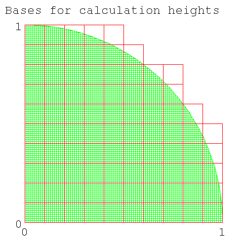
Number of column bases needed for height calculation for num_intervals=10
- Now calculate the volume of each column. Except for the top of the column, which is part of the surface of a sphere, the columns are square columns (with a square base). The volume under the curve has an upper bound, determined by the height of the highest corner of the spherical surface (this corner faces the center of the sphere) and a lower bound, determined by the height of the lowest corner of the spherical surface (this corner faces away from the center of the sphere).
- Now sum the volumes of all the slices. Do this with two loops, one inside the other. The inside loop integrates across each slice and returns the volume for the slice. The outer loop steps the calculation from front to back, each step calculating a new radius for the next slice (and hence the number of intervals in each slice) and summing the volumes from the inner loop.
-
How many iterations do you need for each loop?
Both ways are about the same amount of trouble.
- You could do a variable number of iterations for the inner loop, using a while loop. Since each quadrant has a different number of columns, the while conditional would test if you'd reached the end of the quadrant and then stop.
- You could do the same number of iteractions for the inner loop, using a for loop. The loop variable would range from 0.0..1.0*r. Since only 78% of the columns are inside the octant, 22% of them are outside and have a zero height. Calculating a zero height column for 22% of the columns isn't a big deal, if it simplifies the coding. However you'll still have to test if you're outside the octant before being able to declare a zero height.
| Note |
|---|---|
| End Lesson 30 | |
In this section the students prepared notes, diagrams, and tables for their presentation.
| Note |
|---|---|
| |
The presentation should cover
- How numerical integration works: (you cut up an arbitary shape into many smallers objects - in this case a rectangle - whose area can be calculated. you can use my diagrams if you like.)
- The connection between the area of the quadrant as calculated by numerical integration and the value π.
- How you calculate the upper bound, the lower bound (show code, point out common numbers in both outputs)
- Show how one lot of code can calculate both upper and lower bounds
- Show the increase in precision in the value calculated, as the number of intervals is increased
- Show the (speed) optimisations that you tested, show the speed up from each. Discuss why you used some of these optimisations but not others.
- Show the output as a function of the number of intervals (value calculated, time taken).
- Estimate the upper bound for the error in the output.
- Discuss whether numerical integration is a useful method to calculate π (include time needed to calculate to 15, 100 decimal places).
- Compare speed of calculating π by numerical integration with other algorithms (Leibnitz-Gregory, Machin).