Teaching Computer Programming to High School students: An introductory course using Python as the high level language
Copyright © 2008,2009,2012,2015 Joseph Mack, released under GPL-v3.
08 Jul 2015
Abstract
Originally this was class lessons for a group of 7th graders with no previous exposure to programming. The students were doing this after school on their own time and not for credit. My son's school didn't want me to teach the class using any of the school facilities, as they thought it would compete with a class in Java given to advance placement math 12th graders. However I could use the school facilities, if I didn't teach anything which would fullfil a requirement (which I assume meant anything practical). So the class is at my home and is free. Since this is a hobby activity for the kids, I don't ask them to do homework. As they get further into the class and take on projects, I'll be quite happy for them to work on the projects in their own time, but will let them decide whether/when to do this.
Jan 2012: I'm updating these notes to teach in a class of about 20 kids of mixed ages and skills at a saturday afternoon school.
Mar 2015: I'm teaching a young adult.
Material/images from this webpage may be used, as long as credit is given to the author, and the url of this webpage is included as a reference.
Table of Contents
- 1. Intoductory Notes
- 2. Getting files
- 3. Backup
- 4. Software, Hardware and the Operating System (OS)
- 5. binary numbers, the bit (b), byte (B) and word
- 6. Color Representation on a computer display
- 7. binary operations
- 7.1. binary addition
- 7.2. Algorithm and Order of an algorithm, demonstrated using binary addition
- 7.3. Overflow
- 7.4. Binary Multiplication
- 7.5. Binary Subtraction
- 7.6. bc
- 7.7. Hexadecimal
- 7.8. Base 256
- 7.9. Integer Division
- 8. Primitive Data Types
- 8.1. Primitive Data Type: Integer
- 8.2. Arithmetic with Long Numbers
- 8.3. Negative Integers
- 8.4. Range of Integers
- 8.5. Integer Arithmetic in Python
- 8.6. Largest/Smallest Integer in Python
- 8.7. Primitive Data Type: Characters, ASCII table
- 8.8. Primitive Data Type: Real Numbers
- 8.9. Primitive Data Type: Strings
- 8.10. Is it a string or number?
- 8.11. Other primitive data types
- 9. Other Languages
- 10. External Coding Resources (getting help)
- 11. First Python Program(s) (in Immediate Mode)
- 12. Editor: writing and saving programs
- 12.1. Available Editors
- 12.2. Saving Files: where to put them
- 13. Executing a program
- 14. Variables
- 15. Conditional Evaluation
- 16. Iteration
- 16.1. Iteration Basics
- 16.2. simple for loop
- 16.3. another simple for loop
- 16.4. iterating over a range
- 16.5. the fencepost error
- 16.6. tossing balls at milk bottles: perms and coms
- 16.7. while loop
- 17. Subroutines, procedures, functions and definitions
- 17.1. Function example - greeting.py: no functions, greeting.py
- 17.2. Function example - greeting_2.py: one function, no parameters
- 17.3. Problems with python indenting
- 17.4. Separation of function declaration and function definition: order of calls to functions
- 17.5. Function example - greeting_3.py: one function, one parameter
- 17.6. Scope - greeting_4.py
- 17.7. Code execution: Global and function namespace
- 17.8. Function example - volume_sphere(): function returns a result
- 17.9. Checking Code
- 17.10. Using Math Libraries
- 17.11. Function Documentation
- 17.12. Return Value
- 17.13. Function properties
- 18. Modules
- 18.1. volume_sphere() as a module: writing the function for a module
- 18.2. volume_sphere() as a module: the global namespace code
- 18.3. Code Maintenance
- 18.4. Functions: recap
- 18.5. Function example: volume_hexagonal_prism()
- 18.6. making a module of volume_hexagonal_prism()
- 18.7. Do the tests give the right answers?
- 18.8. Code clean up
- 18.9. Train Wreck code
- 19. Giving a Seminar
- 20. Structured Programming
- 21. Recap
- 22. Back to basics: Real Numbers
- 22.1. Floating point representation of real numbers
- 22.2. Examples of binary floating point numbers
- 22.3. Normalisation of floating point numbers
- 22.4. The 8-bit set of normalised reals
- 22.5. The non-existance of 0.0, NaN and Infinities
- 22.6. Reals with a finite decimal representation, don't always have a finite binary represention
- 22.7. Do not test reals for equality
- 22.8. Floating point precision: Optimisation
- 22.9. Representing money
- 23. Problems resulting from a finite representation of reals
- 24. Two Algorithms: square root, numerical integration
- 25. Calculating square root
- 25.1. Python reals are 64 bit
- 25.2. Babylonian Algorithm
- 25.3. Code for Babylonian Algorithm for Square Root
- 25.4. Order of the Algorithm for calculating the square root
- 25.5. Benchmarking (speed) comparision: Babylonian sqrt() compared to built-in math library sqrt()
- 25.6. Running time comparision: Python/C
- 25.7. Presentation: the Babylonian Square Root
- 26. Numerical Integration
- 26.1. Calculating π by Numerical Integration
- 26.2. an estimate of running time (back of the envelope calculation)
- 26.3. range()/xrange() and out-of-memory problem
- 26.4. Optimising the calculation
- 26.5. Safe Programming with normalised (reduced) numbers
- 26.6. For a constant, multiply by reciprocal rather than divide
- 26.7. add optimisations
- 26.8. Finding π from the upper and lower bounds
- 26.9. calculation of π by numerical integration and timing the runs
- 26.10. Order of the algorithm for calculating π by numerical integration
- 26.11. Errors in the calculation of π by numerical integration
- 26.12. Other algorithms for calculating π
- 26.13. speed of calculation of π by the library routines
- 26.14. Why use Numerical Integration?
- 26.15. Area under arbitrary curve
- 26.16. Calculating the Length of the circumference by Numerical Integration
- 26.17. Calculating the Volume of a Sphere by Numerical Integration
- 26.18. Presentation: Numerical Integration as a method to calculate π
- 27. Arrays
- 27.1. Introduction
- 27.2. Multidimensional Arrays: Operating on Images
- 27.3. Multidimensional Arrays represented by a 1-D array
- 27.4. Array Operations: converting between index and row,col
- 27.5. Array Operations: A better version of row_len, col_len
- 27.6. Array Operations: on rectangular arrays
- 27.7. Image Transformations: rotating a set of pixels
- 27.8. Image Transformations: invert top to bottom
- 27.9. Arrays: access in row and column order
- 27.10. Image Transformations: invert left to right
- 27.11. Arrays: Commutative Operators: inversions and self inverses
- 27.12. Image Transformation: Rotation by multiples of 90°
- 27.13. Commutative Operators: rotations and inversions
- 27.14. Arrays: Using Constants
- 27.15. Arrays: Rotating a Rectangular Image Pt1 (and removing global variables)
- 27.16. Arrays: Rotating a Rectangular Image Pt2 (and removing global variables)
- 27.17. Arrays: Turning reals into an list of int or an array of char (string)
- 28. Templates and Useful Info
- 28.1. Documentation
- 28.2. Random Numbers
- 28.3. Global Variables, User Defined variables and Constants
- 28.4. Simple Lists
- 28.5. List of Lists
- 29. Back to basics: Integer Division
- 30. Joe's Sage Advice
- 30.1. On getting a job
- 30.2. Procedural/OOP programming
- 30.3. Working for Managers
- 30.4. Sitzfleisch
- 31. Review Material
- 31.1. Review: binary
- 31.2. Review: primitive data types
- 31.3. Review: Programming Practices
- 31.4. Review: Conditionals
- 31.5. Review: Iteration
- 31.6. Review: Functions
- 31.7. Review: Modules
- 31.8. Review: Real Numbers
- 31.9. Review: Arrays
The notes here are being written ahead of the classes. I've marked boundaries of delivered classes with "End Lesson X". Each class is about an 90mins, which is about as much as the students and I can take. After a class I revise the material I presented to reflect what I had to say to get the points across, which isn't always what I had in the notes that the students saw. Material below on classes that I've given will be an updated version of what I presented. Material below on classes I haven't given, are not student tested and may be less comprehensible.
The big surprise to me is that when you're presenting new material, the students all say "yeah, yeah we got that" and want you to go on. However when you ask them to do a problem, they haven't a clue what to do. So most of my revisions to the early material were to add worked problems. I also spend a bit of time at the start of the class asking the students to do problems from the previous week's class.
I've found that when asking the students to write a piece of code that some of them (even after almost a year) can't turn a specification into code. Instead I have to say "initialise these variables, use a loop to do X, in the loop calculate Y and print out these values, at the end print out the result". Usually these steps will be given in a list in the notes here. Once I'd shown the students how to initialise and write loops, I had expected them to be able to parse a problem into these steps without my help. However some of them can't and I changed my teaching to reflect this.
The kids bring laptops do to the exercises and they display this page by dhcp'ing and surfing to my router where this page is also stored.
Students are using Mac OS, Windows XP and Linux. For WinXP, the initial lessons used notepad and the windows python. For material starting at the Babylonian square root, I changed the WinXP student over to Cygwin (still using notepad).
In later sections I started having the kids do a presentation on what they'd learned. The primary purpose of this was to accustom the kids to talking in front of groups of people. They also had to organise the material, revealing how much they'd remembered and understood it. The presentation on numerical integration only took 3 classes to cover the material, that it took about 10 classes and homework to assemble the presentation. For the next section of work, I'll have them do presentations on smaller sections of the material, and then have them present on the whole section at the end. I've put most of the answers to questions in footnotes (so students won't see the answers easily during class). However later, when the students are scanning the text to find the important parts for their presentations, it's hidden (in the footnotes). I don't know what to do about that.
- You will need a working installation of python. If you don't already have python on your machine, go to python download (http://www.python.org/download/) and download and install a version of python for your machine.
- To write programs, you will need a programming editor (not needed for the first part of the class).
You will need some standard unix utilities e.g. bash shell and bc if you want to do some of the exercises. bash is the default shell for Linux and is used to retreive/manipulate/input/output information from the computer about its state/condition. bash is run within a terminal (e.g. xterm or a console). bc does arithmetic in different bases (e.g. binary and hexadecimal).
- Linux has bash and bc by default.
- Mac OS/X Jaguar has tcsh by default, Panther has bash by default. Here's an article on installing and running bash on Mac OS (http://www.macdevcenter.com/pub/a/mac/2004/02/24/bash.html).
To run these unix utilities on windows, you will need Cygwin (http://www.Cygwin.com/) plus a few files (the basic install just installs Cygwin). Start with setup.exe (at bottom, "Install or update now!") and select a download site. You will get an initial menu from which you choose your download/install. The menu is not particularly obvious. You will need bash from "shells", bc from "math" or "util".
Cygwin is a unix like environment for windows. It's designed for people who know unix and who are forced to work on windows machines. In this class you can choose your OS, so if you're working under windows, you'll be doing so because that's what you want. In this case you should use the version of python for windows. (It would be possible to use the cygwin version of python instead of the native windows version of python and do all of the class within cygwin).
If you're at a terminal and don't know your shell, type
echo $SHELL
/bin/bash
- Python Tutorial on-line (http://docs.python.org/tut/), Python Tutorial in several formats (http://docs.python.org/download.html).
- LiveWires python teaching course (http://www.livewires.org.uk/python/home). I will be using some of the course as examples.
- LiveWires worksheets (http://www.livewires.org.uk/python/worksheets)
- LiveWires package (http://www.livewires.org.uk/python/package)
- pygames (http://www.pygame.org/download.shtml)
- David Handy (who I find lives close by me) and is a member of Triangle ZPUG (http://starship.python.net/mailman/listinfo/triangle-zpug) has written Computer Programming is Fun (http://www.handysoftware.com/cpif/) to teach python to home schoolers (i.e. kids about the age of my class). I only knew about the LiveWires course when I started this course. David's book has graphics and audio libraries which will add some fun for kids, who don't want to start with hard boiled code and provably correct constructs.
- While looking for clues on validating user input I found CS 107:Computing, Robots, and Python (http://www.cs.usfca.edu/~wolber/courses/107/)
If you're going to be using a computer you need to understand
- Mechanical items/physical objects degrade with time. Moving mechanical items (like hard disks) degrade even faster. All hard disks are guaranteed to fail. Any file residing on only one hard disk cannot be regarded as permanently stored: you cannot rely on the file being there tomorrow.
- Hard disks fail slowly enough that you can store a file on two independant disks and expect that only one of them will fail at a time. What does independant mean? Both disks must be in separate physical locations (you can't lose,drop or damage them both at the same time, they both can't be erased at the same time, be consumed in the same flood/fire). A good first step is to copy new files for a project onto a flash disk at the end of each work session.
- If you fool with your computer enough, eventually you'll wind up wiping/trashing your disk (everyone does this; trashing your disk isn't neccessarily incompetence - but not having a backup is incompetence). Hard disks are cheap enough that you should have a duplicate disk as a bitwise copy of your machine's disk (make sure it's updated often enough that you can afford to loose the updates). When you trash your hard disk, just pop in the backup and use it to rescue your trashed disk. Buy an external usb disk enclosure copy from your current hard disk to the back and later when you need to reverse the process, to recover your disk. Also keep on hand some Linux liveCDs to recover from disk problems. Check that your backup disk works (check that it boots OK at least for your first backup).
- You should plan for the possibility that you will drop or loose your laptop or it will just stop working for no reason at all.
Always keep a copy of the partition table on some (or several) other machine(s). Assuming you boot off /dev/hda (it may be /dev/sda. do the following
dd if=/dev/hda of=/your_flash_disk/mbr.$my_machine_name.$my_kernel_version.hda.$year$month$day |
(and do the reverse to restore your partition table).
Always keep in the back of your mind "how long will it take me to recover if this machine/disk stops working right now?". It shouldn't be much more than grabbing the backup disk off the shelf and updating it with files from your flash disk.
So go buy and start using flash disks as backup for your day to day work. For month to month backup, get an extra hard disk in an external enclosure that allows easy retrieval of the disk.
A computer can be logically divided into
- hardware - the physical parts of a computer, that you can thump/kick. These include, cpu, ethernet cards, harddisks, memory.
software/program - a set of instructions that tell the hardware what to do. software can be in lots of places
- on media (harddisk, floppy disk, flash stick)
- in the computer's memory (when the software is running)
built into ROM (read only memory) in hardware.
software built into hardware that is burned into a ROM and which can't be changed (or changed easily) is called firmware. e.g. a harddisk uses programs in its ROMs to allow it to read/write to disk.
in many formats
- in text form which needs to be compiled before it runs on the computer
- in binary form which will run directly on a computer.
A particularly important piece of software is the operating system (OS). examples are Linux, MacOS, Windows. The purpose of the OS is to virtualise the hardware.
virtualise: make all hardware appear the same to the user, programs, no matter what piece of hardware is being used underneath.
If you use a harddisk that's IDE, SATA, scsi made by any manufacturer, of any size, the OS will present the harddisk as a storage accessed by the same instructions. The instructions will be different for each OS, but once you've picked your OS, the instructions for accessing the harddisk will be the same no matter what harddisk is in the machine.
Computers have millions of pieces of hardware (memory/registers) that are in one of two states
- up/down (N/S) (magnetism, harddisk)
- switch on/off
- voltage high/low
- current high/low
These states are represented by 0/1
You don't have to know what the hardware is doing or even what the hardware technology is, or whether a 0 is represented by high or low voltage. You (or the computer) will just be told that the particular piece of hardware is in the 0 state or the 1 state.
Some hardware maintains its state without power e.g.
- floppy disks
- harddisks
- flash memory
Most hardware looses its state when switched off e.g.
- RAM (random access memory in the computer)
how much memory is in a typical hard disk, flash disk, floppy disk, RAM [1] ?
Since there are only two states (two = bi), the state is represented by a binary digit (called a bit). A bit then either is 0 or 1.
The number system in common daily use is called decimal. The base of the decimal system is 10. The decimal system is used because we have 10 fingers. The hardware in a computer only has two states (0/1), so a computer uses the binary system. There are no decimal numbers inside a computer. Binary numbers are transformed by software to a decimal representation on the screen for us. Number systems used in computing are
- base 10: decimal - for input and output to users
- base 2: binary - the representation used for numbers inside a computer
- base 16: hexadecimal - a more convenient representation of binary for humans.
- base 256: (one byte) used for assigning internet addresses.
bit, wikipedia (http://en.wikipedia.org/wiki/Bit).
Before launching into binary numbers, lets refresh our memories on the positional nature of the representation of decimal numbers.
102=1*100 + 0*10 + 2*1 =1*10^2 + 0*10^1 + 2*10^0 |
The value represented by each digit in the number 102 depends on it's position. The "1" represents "100". If the "1" was in the rightmost position it would represent "1". Each time a digit moves 1 place to the left, it increases the number it represents by a factor of the base of the number system, here 10. The left most digits represent the biggest part of the number.
Let's figure out formally what the decimal number 102 represents. This exercise is trivial, but it will be used next for the binary system. We assemble a list of the powers of the base of the system (the base here is 10, and powers of the base are 1=10^0, 10=10^1, 100=10^2...).Then starting with the smallest number in our list 1 (then 10, then 100...), we look for the first power of 10 that's bigger than our number 102. This is 1000. Then we go back by one member in our list arriving at 100. Next we divide our number (102) by 100.
102/100 = 1 remainder = 02 |
The answer is 1 with a remainder of 02. We repeat the process on the carry, with the next smallest power of 10, in this case 10.
02/10 = 0 remainder = 2 |
We repeat the process, dividing by 1, to get a carry of 0 and we're done
2/1 i = 2 remainder = 0 |
From this we find
102 = 1*100 + 0*10 + 2*1 |
binary numeral system, wikipedia (http://en.wikipedia.org/wiki/Binary_numeral_system).
In a binary number, the base is two, so the number prepresented by each position increases by a factor of 2 as you move left in the number. In binary, you need two numbers to represent all the available values. Here are the two numbers and their decimal equivalents. We see that 0 and 1 are the same in the binary and the decimal system. (You may wonder if this is obvious or trivial or why I'm even saying it. Some of the numbers will be different in the decimal and the hexadecimal system, so wait till we get to the hexadecimal system.)
binary decimal 0 = 0 1 = 1 |
Here's a binary number. Since the base is 2, here's what it represents.
1101 = 1*2^3 + 1*2^2 + 0*2^1 + 1*2^1
     = 1*8   + 1*4   + 0*2   + 1*1
|
As with decimal, the left most digit carries the most value (in 11012, the left most digit represents 810).
What is the decimal representation of 11012?
1101 = 1*2^3 + 1*2^2 + 0*2^1 + 1*2^1
     = 1*8   + 1*4   + 0*2   + 1*1
     = 13 decimal
|
leading zeroes behave the same as for decimal numbers so
00=0 01=1 01101=1101 |
Here's some more binary numbers with their decimal equivalent
  binary decimal
      10=2
      11=3  (2+1)
     100=4
     101=5  (4+1)
    0101=5
00000101=5
    1001=9  (8+1)
    1011=11 (9+2,8+3))
   11011=27 (16+11, 24+3)
   11111=31
|
what is 10112 in decimal [2] ?
Let's go the other way, converting decimal to binary
what is 710 in binary? Do it by stepwise division.
Start with the power of 2 just below your number. Take a guess. 2^3=8. This is bigger than 7. Try next one down. 2^2=4. This is less than 7. Start there 7/4=1, remainder=3 do it again, the power of 2 just below 3 is 2 3/2=1, remainder=1 with the remainder being 0 or 1, we're finished 7=1*2^2 + 1*2^1 + 1*2^0 7 decimal = 111 binary |
In the above exercise, would anything have gone wrong if you'd started dividing by 8 rather than dividing by 4? No, you would have got the answer 710=01112. The leading zero has no effect on the number, so you would still have got a right answer, you just would have done an extra step.
what is 1510 in binary? [3]
You ocassionally need to convert between decimal and binary. Many languages have built-in facilities for doing this.
Here's python code to convert decimal to binary (http://www.daniweb.com/code/snippet285.html). You'll need to know more about programming to use this.
Here's bash code to convert binary to decimal. If you aren't already in a bash shell, start one up in your terminal with the command /bin/bash. On windows, click on the Cygwin icon to get a bash prompt. (comments in bash start with #). The code here is from Bash scripting Tutorial (http://www.linuxconfig.org/Bash_scripting_Tutorial) in the section on arithmetic operations. (Knowing that bash can convert binary to decimal, I found this code with google using the search terms "convert binary decimal bash").
declare -i result #declare result to be an integer result=2#1111 #give result the decimal value of 1111 to base 2 echo $result #output the decimal value to the screen 15 # same code in one line declare -i result;result=2#1111; echo $result 15 |
Python can do the conversion directly for you (example at convert decimal to binary in python http://stackoverflow.com/questions/3528146/convert-decimal-to-binary-in-python). Fire up the python interpreter
python >>> |
Then enter the following string followed by a carriage return. This converts 1610 to binary.
python >>> bin(16) '0b10000' |
The prefix "0b" is python's way of saying the following number is binary. Convert from binary to decimal
>>> 0b1001 9 |
There's often several ways of doing the same thing in a language. Here's another in python from easy binary-decimal-denary conversions in python (http://movingtofreedom.org/2010/10/28/easy-binary-decimal-denary-conversions-in-python-2-6/)
>>> int ('1001', 2)
9
>>> int ('1001', 10)
1001
|
The second number is the base. The output is decimal.
In the previous section, I showed bash code I found on the internet. When writing a new program, you'll often need some functionality that's already been coded up (after 50yrs of computing, there's a lot of code available) that's available in books or on the internet. Books on any computer language will have lots of worked examples. It's often faster to find debugged and working code, than it is to write it yourself from scratch. You're expected to do this and everyone does it. For a class exercise, you may have to nut it out yourself, but when it comes to writing working code, you borrow when you can. When you use someone else's code, you should document where you got it.
- it's the right and honourable thing (TM) to do
- it will be easier to find the original author, if you need to find out more about the code later
- people will be happy to send you more of their code when you ask for it.
- unless you're known to be a superhuman coding fiend, no-one will believe you wrote it all yourself and your credibility will be zero.
- you don't want people who are paying for your coding output, to think you were stupid enough to write it all yourself when working and tested code for that function was already available.
byte, wikipedia (http://en.wikipedia.org/wiki/Byte).
It turns out to be convenient (hardware wise) to manipulate bits in groups of 2n (e.g. 2,4,8,16,32,64,128) bits. For manufacturing, if you wanted to make something bigger, you make another copy of the piece of hardware next to the old piece, leading to increases in hardware in steps of 2. 8 bits is called a byte(B). Initially computer displays were text only and to display numbers, punctuation and letters (both lc and UC) you needed to be able to describe about 80 characters. An 8 bit (1 Byte) counter can handle numbers from 0..255 and can hold enough (80) numbers to represent standard text. A 4 bit counter (0..15) is too small to hold text. Because of the requirement for computers to manipulate characters, the byte became the standard size grouping of bits to manipulate at one time.
some 1Byte numbers expressed in decimal
byte decimal 00001000=8 00001111=15 00010000=16 00100000=32 01000000=64 10000001=129 11111111=255 |
The convention for the integer value of a byte that represents a character is called ASCII (http://en.wikipedia.org/wiki/ASCII) (the American Standard Code for Information Interchange). Here are some byte values for ASCII
byte hexadecimal decimal ASCII 00110000 0x30 48 '0' 00110001 0x31 49 '1' . . 00111001 0x39 57 '9' . . 01000001 0x41 65 'A' 01000010 0x42 66 'B' . . 01011010 0x5A 90 'Z' 01100001 0x61 97 'a' . . 01111010 0x7A 122 'z' |
Single quotes are used to denote a character e.g. 'A'. If you see an 'A' on your screen, the value stored in memory will be 010000012 == 6510.
There is a difference between a character and a number. A character is a glyph (arbitary shape) on a screen. The character '0' is a glyph used to represent the value 0. If the computer wants to store the value 0, it stores 000000002. If the computer wants to write the character '0' on the screen, it's stored as 001100002. The program accessing the memory knows whether the storage represents a number or a character (or something else) and interprets it appropriately. The character 'Z' is stored in the machine as 010110102. 'Z' is not the value 9010.
Let's say the computer is storing the number 101000002=16010=A016. If the user asks the computer to display the number in decimal format on the screen, the frame buffer will contain '1','6','0' i.e. 00110001,00110110,00110000. If the user asks the computer to display the number in hexadecimal format, i.e.'A','0', the frame buffer will contain 01000001,00110000.
The only difference between the binary representation of UC and LC characters is that the 3rd most significant bit (00x00000) is flipped. This simplifies changing between UC and LC.
Convert the following decimal numbers to binary
3 14 27 72 |
Convert the following binary numbers in decimal
11 101 1100 10110110 |
Bytes are always 8 bits. However data is shifted around the computer according to the bus width of the computer (the number of wires/connections between the CPU and the rest of the computer). Most PCs (in 2008) were 32 bit machines, meaning that the CPU manipulates 4 bytes (32 bits) at a time. Since these machines are running at somewhere between 100MHz and 2GHz, then they are doing between 400 and 8000 million byte operations/sec. A 32 bit computer has 32 bit registers and 32 lines for addressing and fetching data. It can transfer data and instructions 4 bytes at a time. In 2012, many PCs are now 64bit machines. The term word comes from the HPC (high performance computing or supercomputers) world, where 64 bit computing has been the standard for 30 yrs, describes the width/size of a piece of data/instruction. In the HPC world, there are words of all sorts of lengths, including 128-bit. A 32-bit computer has a 32-bit (4 byte) word size. A 64-bit computer has a 64-bit (8 byte) word size.
On a 32-bit machine, what is the largest integer that you can represent? [4] You can use python to calculate this for you.
>>> 2**32-1 4294967295L |
A 32-bit machine can generate 4G different numbers (0..4G-1). If the computer uses these numbers as addresses, the computer than can address 4G different objects.
The way computers are built, memory is addressable as bytes. The machine reads or writes the whole byte at a time.
 | Note |
|---|---|
| While the reads and writes to memory occur in bytes, once the byte is fetched into the CPU, the bits can be changed individually. | |
What is the largest amount of memory that a 32-bit computer can address? [5]
How much memory is on your computer? In Windows do control panel->system.
A computer reads and writes to the hard disk. The computer accesses the hard disk in blocks. On PCs the block size is fixed for a particular machine and is 512-4096 bytes. (For Windows, the default block sizes are at Default Cluster Size http://support.microsoft.com/kb/314878. In Windows you can find the block size for your computer by running chkdsk C:. This will take a few minutes, and at the end the computer will display the block/sector size.) When a computer reads or writes to the hard disk, it reads or writes a block as one unit. A computer does not read or write parts of a block.
What is the maximum amount of storage a hard disk can have on a 32-bit computer if the block size is 512 bytes? [6]
Calculate this number with python.[7]
How much storage do you have on your hard disk? To find this in Windows go to explorer, then the properties of your disk.
The information displayed on the computer display is stored in separate memory on the video card. The display is made up of pixels (pixel = picture element i.e. the dots on the screen). Early PCs did not have a lot of video memory and the displays were monochrome. The eye can differentiate about 200 different intensities of light. In grayscale (http://en.wikipedia.org/wiki/Grayscale), on the right hand side at the top, look at the 16 level grayscale. How many bits are needed to represent a 16 level grayscale? [8] If the shading is more than 200 different intensities, the grayscale will appear to be continuous to the human eye. How many bits will you need to make a continuous grayscale? [9]
In the following, give the answer in bytes, using appropriate prefixes.
- What about a 32-bit computer makes it a 32-bit computer?
- What is the maximum amount of byte addressable memory on a 32-bit computer?
- How much memory does your computer have?
- What is the maximum amount of storage on a hard disk with 512 byte sectors on a 32-bit computer?
- How much disk capacity do you have on your computer?
- Determine the sector size of the hard disk on your computer. Calculate the maximum amount of hard disk storage with that sector size on a 32-bit computer.
- Early computer displays were text only, displaying lines that were 40char wide * 25 lines high. How many bytes are necessary to store a character? The information necessary to display the screen is stored on the video card in a piece of memory called the frame buffer. How much frame buffer is needed to store the information for a 40*25 text screen?
- What is the amount of storage required for a pixel that shows a continuous gray scale on a black and white screen? If the display is 1024*786 pixels (a common display size), how much memory does the frame buffer need?
The early computer displays were monochrome and text only. Being text only, the computer hardware could only render letters of a certain type and size. Eventually color displays capable of displaying graphics became available. In a graphics display, every pixel on the screen can be independantly adressed. On a graphics screen you can draw arbitary shapes, e.g. a circle, while on a text only display, you can only display letters that are built into the hardware.
On a computer, color is composed of 3 channels; red, green, blue (r,g,b) allowing the display to present most of the colors in the rainbow and their combination. If you look at a white pixel on a computer display with a 5X magnifying glass, you will see the (r,g,b) subpixels. What is their physical arrangement (i.e. what do you see) [10] ? How many pixels are on your display (in Windows, Control Panel->Display. You'll get the w*h in pixels.)?
Digital and analogue cameras and TV sets all use the same (r,g,b) method of generating colors. This is because the human eye has 3 color receptors, which are also (r,g,b). The color receptors are in the retina and they're called cones. The sensitivity of the three types of cones, as a function of wavelength, is shown in the graph at Mechanism_of_trichromic_color_vision (http://en.wikipedia.org/wiki/Trichromacy#Mechanism_of_trichromic_color_vision). Note that the red and green cones overlap in wavelength, while the blue has little overlap. Light of 500nm will activate all three cones (S,M,L). The unit on the x-axis is what [11] What is the shortest and longest wavelength that humans can see [12] ? You can call these cones the r,g and b cones, if you like, and many people do, but people who study vision call them the S,M and L cones (short, medium and long wavelength). Red has the longest wavelength, while blue is the shortest.
To get an idea of the color at each wavelength, look at the diagram labelled "Relative brightness sensitivity of the human visual system as a function of wavelength" at Color_vision (http://en.wikipedia.org/wiki/Color_vision).
Here's an explanation of the rgb color model (http://en.wikipedia.org/wiki/RGB_color_model). To explore the combinations of colors, using the rgb model, look at color cube (http://www.morecrayons.com/palettes/webSmart/colorcube.php). (The color cube is an idea of Maxwell.)
In the rgb model the color is described by 3 numbers running from 0 (no color) to 1 (full color). Thus (r,g,b)=(1,0,0) is red (abbreviated 1,0,0). White is (1,1,1). (r,g,b)=(1,1,0) has full red and full green but no blue. What color is (1,1,0)? Try a few other combinations. The pairwise colors (1,1,0), (1,0,1), (0,1,1) have common names. What are they? [13] What is (1,1,1)?
If you wanted to present to the user all colors in continuous tones, how much memory would a computer need to store a pixel [14] ? It's convenient hardware-wize to manipulate bytes in groups of 2^n. In this case computer manufacturers use 4 bytes for each pixel, the 4th byte being used for transparency. A typical computer display is 1024 pixels wide * 768 pixels high. How much memory is needed to display full color on this screen [15] ? Modern video cards have lots more memory than this. It's used to store intermediate results when calculating the intensity of pixels.
If you want to look at how colors used to look on computers before full color displays became available, look at monochrome and rgb palettes (http://en.wikipedia.org/wiki/List_of_monochrome_and_RGB_palettes).
When you looked at your computer display, you might have noticed that the blue was darker than the r,g. This is because only about 5% of the sun's (white) light is blue. Thus the color we see as white is (r,g,b)=(45%,50%,5%). If there's any more than 5% b, the color looks blue, rather than white. When we recreate white, we don't need much b, just 5% of the total energy.
If you look at a color (e.g. blue, for long enough (30-60secs), the cones will become bleached (respond less to that color). If you then move your focus to a white area, you will see the complementary color (in this case you'll see white without the blue, e.g. only the red, and green = yellow). As an example follow the instructions on after image (http://www.yorku.ca/eye/afterima.htm).
The cones are relatively insensitive to light and only function in daylight. We have another light receptor, called a rod, which sees black/white/gray only. Rods are most sensitive at 498nm (green). Here is the light sensitivity of rods and cones (http://www.yorku.ca/eye/specsens.htm). The rods are more sensitive to light than are cones. At night only the rods are being use (this is why night scenes have little color). Despite what this curve shows, due to the much greater sensitivity of the rods, the rods detect light beyond the red and blue ends detected by the cones. Thus the color seen at the two ends of the rainbow is grey.
- How much storage is required to represent the intensity of a pixel used to represent a continuous grey scale?
- What is the name of the part of the eye that has the receptors for vision?
- What is the name of the color receptors?
- What is the name of the color independant (gray) receptors?
- Which receptors are responsible for most of our vision at night?
- How much storage is required to represent the color of a pixel used to represent a continuous colored scene?
- What is the name of the colors seen for the following rgb values: (0,0,0), (1,0,0), (0,1,0), (0,0,1), (1,1,0), (1,0,1), (0,0,1), (1,1,1)?
It's important to differentiate a colored light from a colored pigment. A red colored light emits red light (about 650nm). A green colored light emits green light (about 550nm). If you mix both lights together (with a prism, or by shining both on a piece of white paper), you will see both colors together, which the brain interprets as y. Thus lights are additive (r+g=y). For an image of adding lights see RBG illumination (http://en.wikipedia.org/wiki/File:RGB_illumination.jpg) or additive color (http://en.wikipedia.org/wiki/File:AdditiveColor.svg).
On the other hand, a red colored pigment (e.g. paint, printed dye on paper) reflects red. It reflects red, because when illuminated by white light, it absorbs the green and blue. Thus pigments are subtractive (http://en.wikipedia.org/wiki/Subtractive_color). If you mix red and green pigments, the red absorbs g,b, while the green absorbs r,b. All colors will be absorbed and none will be reflected. Thus the mixture of green and red pigments, when seen with white light, will be black (in practice they'll be a dirty dark color, because the pigments don't absorb all light).
What will happen if you mix c and y pigments [16] ?
Color printers use (c,m,y) dies, which are called the primary subtractive colors. You can't make a very good black by adding (c+m+y), so printers use have black (k) too (the symbol b being taken by blue). (As well b ink is cheaper than using up your c+m+y inks.) A printer then is (c,m,y,k).
The primary lights then are (r,g,b). The primary pigments are (c,m,y). When someone says "what are the primary colors?" you have to say "Do you mean primary lights or primary pigments?". (c,m,y are also called secondar lights, but you rarely hear the term used.)
The original experiment of splitting white light into its components with a prism and recombining them, was done by Newton. Newton found that the eye cannot distinquish spectrally pure yellow (produced from a prism) from a combination of red and green (each produced separately by a prism and then combined), even though physically these are distinct ways of creating the color yellow (a prism will show that yellow is still yellow, while the yellow which comes from a combination of red and green, will be split again by a prism into red and green).
To show trichromic vision, I'm now going to do a demonstration with colored light (white light filtered through r,g,b,c,m,y cellophane). If you illuminate a white object, with red light what color will the object appear to be [17] ? If you illuminate a red object with red light, what color will the object be [18] ? If you illuminate a green object with red light, what color will the object be [19] ? If you illuminate a blue object with red light, what color will the object be [20] ? If you illuminate a black object with red light, what color will the object be [21] ?
Now watch the demonstration.
Assume that white is equal amounts of r,g and with 5% b and that the eye isn't terribly sensitive to small changes in brightness. Group r,g,b,c,m,y according to their perceived brightness [22] . Note that c is also perceived as being bright like y (c is used on fire trucks in Chapel Hill, although more likely for political than practical reasons). This is because you can make a color (0.5,1,1) which looks the same to the eye as (0,1,1). Thus you can make a bright c.
The table below shows the perceived color of an object when illuminated by various colors. The r column is filled for you. Fill out the empty columns in this table.
Table 1. Color seen
| object color | illumination | |||||
|---|---|---|---|---|---|---|
| r | g | b | c | m | y | |
| w | r | |||||
| r | r | |||||
| g | k | |||||
| b | k | |||||
| k | k | |||||
The S and M pigments diverged about 500Mya (Trichromic vision in Primates http://physiologyonline.physiology.org/content/17/3/93.full). What geologic age was this, what sort of life forms existed on earth then [23] ?
The big event of the Cambrian, as far as life forms go, was the Cambrian Explosion (http://en.wikipedia.org/wiki/Cambrian_explosion), a period of rapid diversification of life forms and the transition animals from soft bodied to hard bodied. At about 540Mya, trilobites acquired segmented compound eyes (as found in modern arthropods, like insects). Previously trilobites has light sensitive patches, but over a period of about 20My, they developed eyes which could form images, and presumably allow them to locate prey.
Following the aquisition of eyes at 540Mya, it would appear then that by about 500Mya, separate S and M receptors has evolved.
While humans are trichromic, most mammals are dichromic. From Trichromic vision in Primates (http://physiologyonline.physiology.org/content/17/3/93.full).
Exceptions to dichromacy are rare.
Many marine mammals and a few nocturnal rodents, carnivores, and primates have secondarily lost the S cone pigment and become monochromats.
Many diurnal primates, on the other hand, have acquired a third cone pigment, the L cone pigment, which is maximally sensitive to the longer visible wavelengths (red).
The aquisition of the L (red) receptor allowed the primate to differentiate fruit (red, orange and yellow), which constitutes 90% of the diet and young leaves (slightly red), which are eaten as a last resort in the absence of fruit, from the bulk of the green older leaves. At the same time a significant loss of olefactory capacity occured. Presumably it was less risky to spot a ripe fruit with your eyes than to climb a tree and smell the fruit only to discover that it wasn't ripe yet.
Although vertebrates are primitively tetrachromic (many teleost fish, reptiles and birds have four different types of cone cells, each sensitive to distinct light spectra), the mammals are generally dichromic (having only two cone types in the eye). A popular notion is that this reflects a transition to a nocturnal way of life. In the primates, however, trichromic vision has re-evolved - there are three types of cone cell, differentiating colour in the red, green and blue regions of the spectrum. Trichromacy is linked not only to largely diurnal activity, but also to the adaptive advantages of being able to detect coloured fruit and leaves. An important corollary of this argument is that with the shift to acute vision the role of olfaction has become less important. There is probably a lot of truth in this idea, and certainly relative to other mammals (notably the rodents) human olfactory capacity is seriously impaired with many of the relevant genes turned off by being transformed into pseudogenes. (see trichromic vision in mammals http://www.mapoflife.org/topics/topic_328_Trichromic-vision-in-mammals/).
The dichromic vision of mammals may account for their less colorful coats (e.g. cow, moose) compared to birds. From the color of the skins of cartilaginous fish (e.g. sharks), would you expect they have tetrachromic vision as do the telost fish?
Then about 100Mya (lecture) primates acquired trichromic vision (http://mitworld.mit.edu/video/669). Also see Evolution of color vision in primates (http://en.wikipedia.org/wiki/Evolution_of_color_vision_in_primates).
Some human females have tetrachromic vision (http://en.wikipedia.org/wiki/Tetrachromic_vision). Also see tetrachromacy (http://en.wikipedia.org/wiki/Tetrachromacy).
Although beyond the scope of this class, it's worth noting that the brain does not directly receive the (r,g,b) information. The image is subject to neural processing in the retina. (see Trichromic vision in Primates http://physiologyonline.physiology.org/content/17/3/93.full).
The dynamic range over which the eye works is about 107 (day to night). A black road in daylight is emitting more light than does a white sheet of paper indoors, but the brain perceives the road as black, and the paper as white. One mechanism for achieving high dynamic range is encoding intensity of light as the difference between the intensity at the receptor and those immediately surrounding it.
Color is encoded as the difference between b-y and r-g i.e. as a blue-yellow channel and as a red-green channel.
see http://www.yorku.ca/eye/trichrom.htm http://www.yorku.ca/eye/opponent.htm http://www.yorku.ca/eye/huecan.htm http://www.yorku.ca/eye/handj.htm
A computer display is too dim to use in bright light (broad daylight). Let's see what contributes to this.
The computer display is backlit i.e. a fluorescent light at the side(s) of the display illuminates a white sheet behind the display. The white light shines through the pixels, to deliver the light you see. Assume that white light is equal amounts of (r,g,b) (it's not; what are the approximate amounts of energy in each color r,g,b?). Also assume that each (r,g,b) subpixel is the same size.
If a pixel is (1,0,0), what color are we seeing [24] ? How much light is getting through to the viewer? Here's the pixel
---------------------- | | | | | | | | | | | | | | | | | r | | | | | | | | | | | | | | | | | | | ---------------------- |
Only r is on. What fraction of the white backlighting is being presented at the back of the pixel is illuminating the r subpixel [25] ? What fraction of the white light being presented at the back of the r subpixel, is being seen by the user [26] ? What fraction of the white light being presented by the backlight to the whole pixel is being seen by the viewer [27] ? If the pixel was (1,1,1) instead of (1,0,0), what fraction of the backlight would be seen by the viewer [28] ?
At most, only 1/3 of the backlighting gets through, even when the screen is fully white. If you were dichromic (or tetrachromic) with an appropriate TFT display, what fraction of the backlight would get through to you on a white screen?
The simple fix for having a computer display usable in daylight, is to cut out the metal case at the back of the display, allowing sunlight to shine through the TFT pixels. (You will have to be careful not to punch through various protective and functional layers behind the TFT pixels.)
Let's do some binary addition: The rules are the same as for decimal. Here's the addition rules.
0+0=0 1+0=1 1+1=0 with carry, 1+1=10 |
here's the addition rules in table form.
addition carry + | 0 1 + | 0 1 ------- ------- 0 | 0 1 0 | 0 0 1 | 1 0 1 | 0 1 |
| Note |
|---|---|
1+1=0 with a carry. Note: 1+1!=10 (where "!=" is the symbol for "not equal"). The extra leftmost digit, the "1" (as in "1+1=10") becomes the carry digit. It's handled separately by the computer. If you want it, you have to go find it. The equivalent table in decimal for a one digit computer would show that 8+7=5 (and not 15) | |
worked example, working from right to left, one bit at a time
111 (what demical numbers are being added here?) 010 + --- 01 1 carry 001 1 carry 1001 |
What is 1001+00112 [29] ? What decimal numbers are represented?
Algorithm, wikipedia (http://en.wikipedia.org/wiki/Algorithm).
Algorithm: A predetermined sequence of instructions (events) that will lead to a result.
e.g.the algorithm of right-to-left addition will lead to the sum of two numbers.
e.g.the algorithm of putting your books into your school bag in the morning will lead to them all being at school with you the next morning.
What country do we get the word "algorithm"? What does "al" mean? What other words start with "al" used in the same way? [30]
Some algorithms are better (faster, more efficient, scale better) than others. While computers are fast enough that even a bad algorithm can process a small number of calculations, it takes a good algorithm to process large numbers of calculations. Computers are expensive and it's only worth using a computer if you're doing large numbers of calculations. We're always interested in how an algorithm scales with problem size. So we're always interested in the goodness of the algorithm being used.
The measure of goodness of an algorithm is the rate at which the time for it's execution increases as the problem size increases (i.e. how the algorithm scales). If you double the size of the problem, does the execution time not change (independant of problem size), double (linear in problem size) or quadruple (scales as the square of the problem size)?
This change in execution time, as a function of problem size, is called the Order of the algorithm.
- O(1): the execution time is always the same (1), i.e.is independant of problem size
- O(n): the execution time is proportional to the problem size.
- O(n2): the execution time goes up as the square of the problem size (O(n2)) algorithms are too slow to be used for large problems).
Speed (Order) of the addition operation:
Addition of a pair of 1 byte numbers, one digit at a time (as we did above), takes 8 steps. The Order of addition, doing it one step at a time, is O(n) i.e. time taken is proportional to n=number of bits.
There's a faster way: add the bits in parallel and handle the carries in a 2nd step
111 010 --- 101 add 10 carry (note the first carry of 0 is put into the 2nd column from the right) --- 001 add 1 carry ---- 1001 add 0 no carry - we're done |
| Note |
|---|---|
| The last carry/add is done in computer hardware as part of the adding the carry and add so there's really only two steps. | |
Addition done in parallel takes 2 steps, no matter how long the numbers being added. The Order of parallel addition algorithm is O(1) i.e. is proportional to 1 i.e.addition takes the same time independant of the number of bits being added. The O(1) parallel addition algorithm scales better than the O(n) stepwise algorithm.
To do parallel addition, you need to increase the amount of hardware, but you only have to pay for the hardware once and the extra cost can be amortised over the billions of addition operations that will be done during the lifetime of the computer.
What is amortization (http://en.wikipedia.org/wiki/Amortization)?
Amortization is the process of saving money, in a large project, by paying a large amount at the beginning.
An example: Let's say you want to dig a small hole in the ground. The hole can be dug by one person using a shovel in 1hr at a cost of $20. Now let's say you want to dig a hole 100 times bigger. You could hire 100 people with shovels at a cost of $2000. Or you could rent a BobCat ($500) to do the same job. You have amortised the larger cost of the BobCat over the bigger job, saving you money.
Let's say in the design of a computer, you have the choice of two pieces of hardware; a fast expensive piece and a slow cheap piece and the piece you choose only has to be paid for once, and you can use that process as many times as you want. In this case you choose the expensive piece of hardware, and you are said to be amortising the extra cost over the life of the machine.
e.g. cost of stepwise adder=$10. cost of parallel adder=$20. If you're going to be doing 1015 additions before you retire the machine, the amortised extra cost of the parallel adder is 10-14$/addition. Most people will accept this extra cost, because of the increased speed will save them money for each run of the program.
The most common place that amortisation is used in computing is in the cost of writing a program. Writing a program is expensive; you have to pay the programmers salary, benefits, heating/AC, electricity and buy computers and lease a premises to do this. A program may cost $1k-$100M to write. However if the program is run millions of times, the cost/run for the end user may be insignificant compared to the cost of hiring staff and buying machines to run the program. In this case the costs of the programmer's time is said to be amortised over the number of times the program will be run. Because writing programs is so expensive, you only write programs that are going to be run many times.
Here's the time/steps for the two types of addition for different problem sizes
Stepwise Parallel 1 2 2 2 4 2 3 6 2 4 8 2 . . 16 32 2 |
We don't really care what the constant of proportion is, i.e.we don't care if each step takes 1usec, 1msec or 1sec, only how the time to completion scales with problem size. We know that if we scale the problem by some large number (e.g.106), that the constant of proportionality will be swamped by the problem size. As well we don't care if the constant of proportionality is different for each process. Let's say that parallel addition took 8 steps instead of 2. Here's the new times for addition.
bits Stepwise Parallel 1 2 8 2 4 8 3 6 8 4 8 8 . . 16 32 8 |
We only need to get to numbers of length 8 bits to be ahead with parallel addition.
say we have a 4bit computer, what is
1010 0110+ ---- |
[31] ?
This addition results in a digit rolling off the left hand end. Loosing a digit off the left end of the register is called overflow (underflow is loosing a digit off the right end of the register). If you do this addition on a 4bit computer, you'll get an erroneous answer. In some circumstances you'll get an error message on overflow and in other situations you won't. Since overflow is part of the design of a computer, it is expected and is not neccessarily regarded as an error. (A drinking glass will only hold so much fluid. If you put in more fluid, it will overflow. People accept overflow as part of the design of a drinking glass.)
With addition, you have to anticipate getting a number that is 1 bit longer than the two numbers being added. If both numbers have a 1 in the most significant bit, then you'll have overflow.
the rules are similar to decimal - here's the multiplication table (no carry is needed for binary multiplication)
* | 0 1 ------- 0 | 0 0 1 | 0 1 |
Multiplication by 1,10,100 left shifts the digits by 0,1,2...n places (i.e. by adding a '0' on the righthand end). This is the same whether you're working in decimal or binary. Left shifting is a fast operation in a computer. The computer uses left shifting to multiply.
| Note | |
|---|---|---|
what numbers are represented in each case? | ||
Left shifting produces overflow. Assume a 4bit computer
1100* 10=1000 (not 11000) 1100*100=0000 (not 110000) |
If a 0 overflows, you get the correct result.
Computers do multiplication the same way we do, one digit at a time (using left shifting), and adding the results in parallel.
what is
1010 11x ---- 1010 1010 + ---- 11110 addition 0000 carry ----- 11110 |
again
    1010
    1101x
    ----
    1010
   0000
  1010
 1010   +
 -------
 1110010
   1     carry (a couple of rounds)
 -------
100000010

the carries are done in parallel by specially designed hardware.
multiplication is fast and is O(1).
|
what is 10102x01102? [32]
what is 11002x10012? [33]
With addition, as long as you don't get an overflow, the width (number of bytes) of the result (adduct) is the same as the width of the two addends (the numbers you added together). With multiplication what is the width of the product if the two factor are 1 byte in size? [34]
A CPU is setup with appropriate width registers to handle multiplication. When you store the result back in memory, it may be too big. Usually the language that you are using for your coding will handle this for you. We'll see how this works out later in examples.
It is not neccessary to have a separate set of hardware for subtraction. You could in principle add the negative of the number, but we don't have negative numbers. Hardware only knows about 0-255 and has no concept of positive or negative numbers.
| Note |
|---|---|
| Software can interpret certain values of a byte as being negative, but we haven't got that far yet. | |
However we don't need negative numbers for substraction. Instead we add the complement (for binary, it's the two's complement: the two's complement instruction is fast - one clock cycle). Let's find out about the complement.
Let's look at subtraction by adding the complement using a decimal example.
Let's say we want to do
9-3=6 |
and we have a 1 decimal digit (dit) computer. Here's the addition table for a 1 dit computer.
+ | 0 1 2 3 4 5 6 7 8 9 ----------------------- 0 | 0 1 2 3 4 5 6 7 8 9 1 | 1 2 3 4 5 6 7 8 9 0 2 | 2 3 4 5 6 7 8 9 0 1 3 | 3 4 5 6 7 8 9 0 1 2 4 | 4 5 6 7 8 9 0 1 2 3 5 | 5 6 7 8 9 0 1 2 3 4 6 | 6 7 8 9 0 1 2 3 4 5 7 | 7 8 9 0 1 2 3 4 5 6 8 | 8 9 0 1 2 3 4 5 6 7 9 | 9 0 1 2 3 4 5 6 7 8 |
| Note |
|---|---|
| remember, because we have a one digit computer, 9+9=8. (9+9!=18, the 1 is lost by overflow.) | |
If we're going to do the substraction 9-3=6, by adding some number to 9, what number do we add to get 6? Looking at the addition table, we find we have to add 7.
9-3=6 what we want 9+?=6 what we're looking for 9+7=6 the answer from looking up the addition table above |
The ten's complement of 3 then is 7.
What if we want to subtract 3 from any other number, say 8? If we want to do 8-3=5, by adding a number to 8, on looking at the addition table, we have to add 7. So whenever we want to subtract 3, instead we add 7.
8-3=5 what we want 8+?=5 what we're looking for 8+7=5 the answer from lookup up the addition table above. |
We find the ten's complement of 3 is 7 no matter what number we subtract 3 from. Making the complement of a number only depends on the number, not what we subtract it from.
What is the ten's complement of 8?
9-8=1 9+?=1 9+2=1 |
the ten's complement of 8 is 2.
What's the ten's complement of 9?
9-9=0 9+?=0 9+1=0 |
the ten's complement of 9 is 1.
What is the ten's complement of 0, of 4? [35]
Overflow is required to make this process work. Overflow isn't an advantage or a disadvantage; it's just part of the design of a computer. Since we have overflow, we can use it to do subtraction by addition of the complement, rather than having to build a subtractor into the hardware.
Here's the decimal (10's or ten's) complement table
number complement 0 0 1 9 2 8 3 7 4 6 5 5 6 4 7 3 8 2 9 1 |
The complement is the number you have to add to a number to get a sum of 0.
| Note |
|---|---|
| the sum is not really 0; the sum is 10, but the left digit is lost through overflow. | |
The complement of a single digit number then is
complement=(base of the system, here 10)-(the number).
In a 1 dit computer there is no such thing as 10 (you need two digits to make a 10). So the process of subtracting the number from 10 doesn't work. Your computer doesn't have subtraction either. We have to do something else. Instead if you want the ten's complement of 7, you start with your list of numbers in inverse order (9,8..0) and you ask the computer to come in 3 places from the biggest number (here 9), i.e.8,7,6 giving 6. Then you add 1 giving 7.
| Note |
|---|---|
| Subtracting from 10 or marching in from 9 are the same to you, but if you're wiring up a computer, you can't subtract from 10, but you can count in from 9. | |
Summary: if we're going to do 9-3, we add 10 to the -3, giving +7. The answer we'll get by doing 9+7 will be 10 more than what we want. However the extra 10 will be lost through overflow (automatically subtracting 10 from the result), giving us the correct answer.
what we wanted 9-3=6 what the computer calculated (it added 10 to both sides) 9+(-3+10)=10+6 9+ 7 = 6 the answer the computer gave us 6 |
We've done subtraction in decimal using the ten's complement. Now we're going to do subtraction in binary using the two's complement. What is the two's complement of the 2 bit number 012?
find some number that when added to 012 gives 002 (just start poking in numbers till you get the required answer).
01 #decimal 1 11 #decimal 3 ---- 00 Note: overflow is needed to get 00 |
See any connection between 1 and its complement 3, in a 2 bit system [36] ?
A 4 bit number system has base 16. See any connection between the values of the number-complement pairs and a 4 bit number system in the following examples? Using brute force, what's the two's complement of the 4 bit numbers
let's try an example in a regular 8 bit byte. Using brute force, what's the two's complement of 01000110? (for labelling, let's use the words minuend, subtrahend and difference.)
01000101 subtrahend 10111011 complement -------- 00000000 |
How do you make the complement in binary?
Following the decimal examples (above), to get the complement, you count in from the end number (1 or 0) by 1 number (i.e. you flip the bits), shown here
01000101 original subtrahend 10111010 bit flipped subtrahend 10111011 known two's complement |
| Note |
|---|---|
| By looking at the bit flipped number and the two's complement, you can see that you have to add 1 (as is done for the decimal example). | |
10111011 bit flipped subtrahend + 1 |
binary complement=(bit flipped subtrahend + 1)
we've found the complement (the -ve + the base number of the system)
01000101 subtrahend (decimal 69) 10111011 complement (decimal 187) |
What's the sum of the 8 bit subtrahend and its complement [41]
with the complement, we can do the subtraction.
10000000 minuend (decimal 128) 01000101- subtrahend (decimal 69) -------- 10111010 bit flipped subtrahend 10111011 bit flipped subtrahend +1 = complement of 69 |
Do the subtraction by adding the two's complement
10000000 minuend (decimal 128) 10111011 complement of decimal 69 --------- 00111011 difference (left bit overflows on an 8 bit computer) result: binary decimal 10000000 128 01000101- 69- ------- --- 00111011 59 |
using the two's complement to do subtraction, what is
| Note |
|---|---|
| End Lesson 2. Some kids didn't get the material on the complement and didn't complete the excercises. I added more exercises and started Lesson 3 at the beginning of binary subtraction. | |
Most people can only do 4bits of binary in their head. You either go to hexadecimal (below) or use a binary calculator. Fire up a terminal and try a few examples (you can recall the last line with the uparrow key and edit it without having to type in the whole line again).
bc (basic calculator?) is a general purpose calculator. Using a terminal, try some standard arithmetic e.g.(+-/*).
echo "3*4" | bc 12 |
bc does all input and output in decimal, until you tell it otherwise.
- You change the output base using obase
- You change the input base using ibase. After you've run this command, all following input will be read using the new ibase.
Here's a few binary examples.
#input will be in binary, output is decimal since you haven't changed output echo "ibase=2; 1100-101" | bc 7 #with obase explicitly set (not needed if obase is 10) echo "obase=10;ibase=2; 1100-101" | bc 7 #same problem, output in binary echo "obase=2;ibase=2; 1100-101" | bc 111 #convert decimal to binary echo "obase=2; 17" | bc 10001 #other examples: echo "obase=10;ibase=2; 1100+101" | bc 17 echo "obase=2;ibase=2; 1100+101" | bc 10001 |
Exercises: Hint - the number(s) you're processing are in the last instruction on the line. Before you run the instruction, figure out the base for the input and for the output and then decide whether you need to set obase and/or ibase.
The normal order is obase/ibase. What happens if you reverse the order of obase and ibase without changing their values?
normal order echo "obase=10;ibase=2;01110001" |bc 113 inverted order echo "ibase=2;obase=10;01110001" |bc 1110001 |
bc defaults to decimal input. In the normal order, bc interprets obase as 1010 and ibase as 210 (i.e. binary). The input will be intepreted as binary and output will be in decimal. In the inverted order, obase says that all further input will be interpreted as base 210 (i.e. binary). Thus the obase value is 102 (210), i.e. the answer will be in binary.
As long as you know what you're doing, you can use obase,ibase in any order. To minimise suprises, use obase first, leaving the input decimal, then input the value for ibase in decimal.
For the length of numbers used in a computer, binary is cumbersome. Unless you really want to know the state of a particular bit, you use hexadecimal (a number system with base 16), which uses 1 symbol for 4 bits, and runs from 0..f (or 0..F)
binary hex decimal 0000 0 0 0001 1 1 0010 2 2 . . 1000 8 8 1001 9 9 1010 a or A 10 1011 b or B 11 1100 c or C 12 1101 d or D 13 1110 e or E 14 1111 f or F 15 |
When input to a computer is ambiguous as to its value, hexadecimal is represented as "OxF" or "Fh" (preceded by "Ox" or postceded by "h").
Here's conversion of hexadecimal to decimal using bash
declare -i result #declare result to be an integer result=16#ffff #give result the value in decimal of hex ffff echo $result #echo $result to the screen 65535 #or all in one line declare -i result;result=16#ffff; echo $result 65535 |
using bc
echo "obase=16;ibase=16; F+F" | bc 1E |
| Note |
|---|---|
| End Lesson 3. Spent some time in the first half of the class going through the two's complement exercises which I added after lesson 2. I asked the kids to try the following exercises for homework. They didn't do them so I started with the decimal/binary/hex table above and then worked them through the exercises below, at the start of the class. | |
Using any method
- convert 1010 to hexadecimal [48]
- convert 10112 to hexadecimal [49]
- make up the hex addition table and the carry table [50]
- using this hex addition and carry table, give the result of adding "F+F" on a 4 bit computer [51] and an 8 bit computer [52]
- find the sum of cd+0e (both hex) in hex for a 1 byte computer. Do it with bc and then using the table you just derived. [53]
- give the hex complement of the hex numbers: 1,6,3A [54]
- what is FD01-EF56 in hex [55] ?
| Note |
|---|---|
| Base 256 logically belongs here, but since you don't need it to start programming, and the introductory part of this course is long enough, I'll do it some time later. The material is at back to basics, base 256 | |
| Note |
|---|---|
| Integer division logically belongs here, but since you don't need it to start programming, and the introductory part of this course is long enough, I'll do it some time later. The material is at Integer Division | |
Primitive type, wikipedia (http://en.wikipedia.org/wiki/Primitive_type).
Bytes hold numbers 0-25510, 00000000-111111112, 00-FFh It's all the computer is ever going to have. We need to use these bytes to represent things more useful/familiar to us.
Using bytes of 0-255, languages implement a set of primitive data types (and provide operators to manipulate the primitive data types).
- integers:e.g. 42, 1024, -100
characters: e.g. 'a','Z','0',' '
Note This explanation of the difference between '0' and 0 was later in the lesson, but the students immediately protested that '0' was a number and not a character. What's the difference between the integer 0 and the character '0'?
the integer 0:.
If represented by a single byte, it will be 00000000. You can do arithmetic operations (e.g. multiply, add, subtract and divide) with the integer 0.
the character/symbol '0':.
Has particular shape. It's represented by the byte 30h. When the computer needs to draw/print this character on a screen, the byte 30h is sent to the screen/printer, where the hardware knows to draw a symbol of the right shape to be a zero. The computer is not allowed to do arithmetic operations (e.g. add, multiply, subtract or divide) on the character '0'. However the computer can test the variable holding the character '0' to see whether it represents a decimal digit (number), hexadecimal digit, punctuation, letter and if a letter, whether it's upper or lower case.
In situations where the computer doesn't know whether 0 is a number or character, you have to explicitly write '0' and/or "0" (depending on the language) for the character, while 0 is used for the number.
To add to the confustion, the word "number" is used to mean both a numerical quantity and the characters which represent it. Context will indicate which is meant.
I will be talking about the ASCII character set, ASCII, wikipedia (http://en.wikipedia.org/wiki/ASCII), which is useful for simple text in (US) English. An attempt at a universal character set, see Unicode, wikipedia (http://en.wikipedia.org/wiki/Unicode).
Early in the days of computing, the US Govt decided to only buy computers that used the same character set and it mandated ASCII. Until then, manufacturers all used different hexadecimal representations of characters. Because ASCII was required for computers bought by the USGovt from the early days of computing, all manufacturers supported ASCII. ASCII is still the only guaranteed way of exchanging information between two computers. Usually if one computer wants to send the value 3.14159 to another computer, it is sent as a series of characters (string) and transformed into a number at the receiving end. (There is no agreed upon convention for exchanging numbers.) Thus e-mail and webpages all use ASCII. Many computer peripherals (e.g. temperature sensors) send their data as a string of ascii characters (terminated by a carriage return), which is then turned into a number within the computer.
see big government does work.
Note The US Govt could have set standards for exchange of numbers too, but it didn't, so numbers are exchanged between computers by ASCII. real numbers: e.g. -43.0, 3.14159, 98.4
Floating point numbers, wikipedia (http://en.wikipedia.org/wiki/Floating_point).
boolean: e.g. true, false (these are the only two allowed values) (most languages don't have booleans, you have to fake it).
Boolean datatype, wikipedia (http://en.wikipedia.org/wiki/Boolean_datatype). Boolean logic in computer science, wikipedia (http://en.wikipedia.org/wiki/Boolean_logic_in_computer_science).
strings: e.g. "happy birthday", "my birthday is 1 Jan 2000".
String (computer science), wikipedia (http://en.wikipedia.org/wiki/String_%28computer_science%29).
Programs don't usually do much arithmetic with integers. Integers are used as counters in loops and to keep track of the position in an executing program. Integers do come from digital sensors: e.g. images from digital cameras, digital audio, digital sensors. However most data, by the time it arrives at the computer, is reals.
In a 32 bit computer, an integer has a range of 0-4294967295 (232, this number is referred to, somewhat inaccurately as 4G, but we've all accepted what it means - it's the 32 bit barrier).
#in bash #binary declare -i result;result=2#11111111111111111111111111111111; echo $result 4294967295 #hexadecimal declare -i result;result=16#ffffffff; echo $result 4294967295 |
Numbers needing more bits than the machine's register size are called Long (or long), e.g. a 64 bit number on a 32 bit machine. Arithmetic on long numbers needs at least two steps, each of 32-bit numbers, and requires an "add with carry" (ADC) instruction (found on all general purpose computers designed to be able to load any code the user wants to install, but not found on special purpose computers exclusively running preinstalled code such as cell phones, routers, automotive computer chips). Here's how addition of long numbers works. Let's assume a 2bit computer and we want to add a 4bit number.
0010 1011+ ---- ???? |
First split the problem into pieces managable by the hardware (here 2 bits) giving us the right hand half (the least significant bits) and the left hand half (the most significant bits).
LH RH 00 10 10+ 11+ -- -- ?? ?? |
Next a word about addition and carry: When doing addition by hand, for the rightmost digit, there is never a carry (there's no column to its right to produce a carry bit). However since the computer has a carry bit for the other 7 digits, it's simplest to have a carry bit for the right most column, and it's set to 0 at the start of addition. This carry bit is useful for the ADC operation (see below).
RH 10 11+ ---- ?? sum ?0 carry for right colum set to 0 step 1: least significant digit, add two digits + carry digit. The carry to the 2nd column is 0. RH 10 11+ -- ?1 sum 00 carry step 2: 2nd least significant digit, add two digits + carry digit. There is overflow RH 10 11+ -- 01 sum 00 carry (with overflow) |
The computer did 10+112 and got 012 (i.e. 2+3=1, with an overflow of 1 in the 3rd least significant digit, 1002=4).
The computer has a FLAGS register (32-bits in a 32 bit computer), which holds, in each bit, status information about the executing program, including whether the previous instruction overflowed, underflowed or set a carry.
The addition above overflowed, but the computer doesn't know if the bit is required for Long addition, in which case the overflow is really a carry. The computer stores the overflow bit in the carry bit in the flags register just in case. If the computer is doing a Long addition, the next step will ask for the carry bit. If the computer isn't doing a Long addition, then then the carry bit will be ignored (and will be lost).
Here's what the calculation looks like now (only the state of the carry bit is shown in the FLAGS register). The computer will first add the right most digits in its 2bit registers, using the regular add (ADD) instruction, which only adds the two numbers and the information setup in the carry input to the adder.
before 1st addition LH RH FLAGS 00 10 ? 10+ 11+ -- -- ?? ?? sum ?0 ?0 carry after 1st addition LH RH FLAGS 00 10 1 10+ 11+ -- -- ?? 01 sum ?0 00 carry |
Because of the overflow, the FLAGS register is now 1. The computer has been told that it's doing the 2nd step in a Long addition. It uses the "add with carry" (ADC) instruction, which transfers the carry bit in the FLAGS register to the adder, and then does a normal addition.
2nd addition. first step, copy carry bit from FLAGS to carry input for LH LH RH FLAGS 00 10 1 10+ 11+ -- -- ?? 01 sum ?1 00 carry 2nd step, add digits and carry digits for LH numbers LH RH FLAGS 00 10 1 10+ 11+ -- -- 11 01 sum 01 00 carry we now read out the sum digits 11 01 giving the required answer of 1101 |
You can chain addition to any precision (on a 32-bit computer, to 64, 96, 128-bits...) Standard calculations rarely need more than 64 bits, but some people want to calculate π to billions of places and this is how they do it.
Long arithmetic is slower than regular arithmetic. You don't ask for Long operations unless you know you need them.
| Note |
|---|---|
| End Lesson 4 | |
If we wanted negative integers, how would we do it? Pretend you're a 1 byte computer and you need to represent -1. You can do this by finding out the number which added to 1 gives 0.
00000001 ????????+ -------- 00000000 |
The answer is 111111112, 25510or FFh (note: computers need overflow to work).
00000001 11111111+ -------- 00000000 |
You've seen the computer version of -ve numbers before. They're called what [56] ? They are the (-ve of the number + the base) (in a 1 byte computer the base is 256).
What is -210 in binary, hexadecimal? [57]
How do we know whether 255 should be interpreted as -1 or 255?
The level of primitive data types, is one level above a byte. Your program keeps a record of the primitive data type that each particular byte represents. When you write your program, your code will have descriptors stating whether this integer will have +ve only values (called an unsigned int) or both +ve and -ve values (called a signed int). Some programming languages will have already decided that you'll be using a signed int and you won't have any choice.
If you have a signed int, then integers with high order bit=1 are -ve while those with high order bit=0 are +ve.
binary hexadecimal decimal 00000000 00 0 00000001 01 1 . . 01111111 7F 127 10000000 80 -127 10000001 81 -126 . . 11111100 FC -4 11111101 FD -3 11111110 FE -2 11111111 FF -1 |
Linux runs on 32 bit computers. What values is represented by 32x1's (or FFFFFFFF) in Linux bash. On a 32 bit machine we might expect this to be -1.
declare -i result;result=16#ffffffff; echo $result 4294967295 |
This is not a negative number. What's going on? Let's try a 64-bit number (just for reference, the biggest number that can be represented by 64 bits is 264=18,446,744,073,709,551,616=18.45*1018).
declare -i result;result=16#ffffffffffffffff; echo $result -1 declare -i result;result=16#7fffffffffffffff; echo $result 9223372036854775807 declare -i result;result=16#8000000000000000; echo $result -9223372036854775808 |
bash in Linux rolls over to -ve numbers half way through the 64 numbers: the integers in bash on Linux on 32 bit machines are 64-bit signed integers.
| Note |
|---|---|
| see long_numbers for 64-bit math on 32 bit machines. | |
Here is the range of values that various sized integers (int) can represent. To give an idea of the relative sizes, the table shows the time (stored as seconds) represented by that integer.
8bit 16bit 32-bit 64-bit unsigned 0-255 0-65535 0-4294967296 0-18446744073709551616 signed -/+127 -/+32767 -/+2147483647 -/+9223372036854775808 unsigned time 4mins 18hrs 136yrs 584,942,417,355yrs signed time 2mins 9hrs 68yrs 292,471,208,677yrs |
You'll see these numbers often enough that you'll start to remember them. For the moment be prepared to see numbers pop up that you've not previously seen much of.
The Y2.038K problem. In 1999 the computer world was in a flurry: programmers who'd prepresented years in their dates using 2 digits, realised that the year 00 would represent the year 1900. Paychecks would not be processed, elevators would stop working at midnight, trapping thousands (if not millions) of innocent people, and planes would fall out of the sky (except Japanese planes). A bigger calamity could not be imagined. The world's bureaucrats heroically spent millions$ of taxpayer's and consumer's money to prevent certain disaster. On 01 Jan 2000, none of the predicted misfortunes occured, for which we must thank the selfless and unacknowledged taxpayers and consumers of the world.
Unix represents time as a signed 32-bit integer of seconds, starting 1 Jan 1970, this date itself a major blunder [58] . If in Jan 2038, you're still using a 32 bit OS (not likely for desktop machines, but quite possible for embedded devices sitting in computer controlled machinery, which rarely need 32 bits, much less 64 bits), Unix time will overflow in Jan 2038. If in Jan 2038, your computer controlled refrigerator stops ordering food, it will be because the refrigerator is asking for food to be delivered in 1970. Jan 2008 was a good time to take out a 30yr loan for 250,000$; your monthly payments would be -1,600$ (a comment from slashdot in Jan 2008. http://it.slashdot.org/article.pl?sid=08/01/15/1928213).
A 32 bit computer can generate how many different different integers [59] ? This computer then is capable of generating that many different integers. If you use the integers to be labels or addresses, you can label that many different items.
A 32 bit computer addresses its memory in bytes using address lines in the hardware. The computer has to read/write a byte as one unit; it can't address individual bits in a byte in memory - it has to read or write the whole byte. Once the computer has read the byte into a register, then each bit within the byte is separately addressable. What is the maximum number of bytes a 32 bit computer can address, and how much memory is this [60] ?
Not too long ago, microprocessors had 4kbytes of memory. Now for many applications, computers need more than 4Gbytes of memory. These applications all have to be run on 64-bit computers. But if you wanted to increase the amount of memory available to 32-bit computers, how could you do it [61] ?
In fact most data and instructions in a 32-bit computer are 32 bits and are fetched 32 bits at a time, so changing the addressing to 32 bits would not be a big change. A char would now have to be represented by the byte of interest, followed (or preceded) by 3 empty bytes. The instructions that work on chars would have to mask off the 3 empty bytes. Since chars (in most programs) are a small fraction of the data held in memory, these unused bytes would not cause too much wasted space in memory.
I don't know why 32 bit computer manufacturer's didn't go to 32 bit addressing. Possible reasons might be
- Compatibility is a big factor in the commodity market; unless of course you're Apple, who brings out new hardware and software every 3yrs, discontinues support of the current hardware and tells everyone how fortunate they are to be able to buy the new hardware and software. This selects for grateful and well-heeled customers. For the rest of the commodity market, everything has to be backward compatible, back to the clay tablet. The new architecture would break old code. Most people using PCs are running applications on the desktop (business/office applications), and don't have the source code for the programs they run; they run proprietary binaries and would have to buy new versions of their programs if they upgraded to 32 bit addressed hardware.
- Most of a desktop machine's activities are character oriented; typing into a wordprocessor, display on a screen, sending characters or mouse clicks to machines on the internet (all of which have to be sent one character at a time in an IP packet, and have to await a reply packet before being displayed on your screen). (In contrast, an HPC machine doesn't interact with the slow user, keyboard, or screen; it runs for hours, days or weeks and then dumps its output as files, to be poured over later by the programmer/user.)
- 64 bit addressing is available if you need it. 64 bit machines have been around for 30yrs or so. People needing large amounts of memory are crunching large amounts of data. They have more money and aren't running desktop applications. They're either using programs they wrote themselves (i.e. they have the source code, which they can recompile) or are prepared to pay for 64 bit versions of standard programs. They are also prepared to pay for 64 bit machines.
- 64 bit addressing is available for the desktop too. The hardware for the commodity market (PCs) is changing over to 64 bit about the same time as the arrival of desktop programs that handle large amounts of data.
Harddisks read/write data to/from independantly addressable blocks (i.e. the computer cannot address individual bits or bytes within a block; it has to address and then read or write the block as one indivisible unit). Let's assume a blocksize of 512bytes. If the computer wants 1 bit off the harddisk, the computer has to know the address of the block, read the whole 512bytes into registers, manipulate the 1 bit and the write the 512byte block back to disk. What's the maximum number of blocks a 32 bit computer can address on a harddisk and how much can be stored on a disk with blocksize=512bytes [62] ?
If you wanted to put a bigger disk on a 32 bit computer, how would a harddisk manufacturer do it [63] ?
Harddisk manufacturers originally started with block size of 512 bytes and have incremented the size of the blocks continuously over the years. I don't know why hard disk manufacturers can change the blocksize whenever they want and not have programs fail, while at the same time microprocessor manufacturers have not been able change from 8bit addressing to 32 bit addressing. Possible reasons might be
- While the 32 bit barrier for memory was always a long way off and programs never had to change this size, harddisk manufacturers set specs for their disks that were regularly exceeded almost the next year. You'd think the harddisk manufacturers would set a spec that would last 10yrs or so, but they didn't. OS writers were continually virtuallising out new harddisk hardware, while not having to change the word size for fetching from memory.
My guess as why memory addressing stayed constant at the 1 byte granularity over decades, while disk block size (granularity) increased from 512 bytes to 8192 bytes, is that going to larger block size forgoes the chance of addressing a 512 byte block, which doesn't cause any problems (you don't ship disk blocks off the local machine), but choosing 32-bit addressing forgoes the chance to address a byte, which you do want to be able to move around (including sending to other machines or peripherals).
IPv4 internet addressing uses a 32 bit unsigned integer (IP) to uniquely identify each network device (e.g. no two devices/computers can have the came IP). How many devices can be simultaneously on the internet using an IPv4 IP [64] ?
The internet game "World of Warcraft" (reported in slashdot, http://games.slashdot.org/games/08/01/19/1321241.shtml) uses a 32 bit integer to store the amount of gold that players earn. Some players have reached that limit and can no longer receive gold from other players. If these players have 1c of gold for each bit, what is their wealth in $ [65] ?
The world's telephone system carries voice data in 8bit form i.e. it converts your voice into bytes, each byte representing the amplitude of your voice at any instant. How many different amplitude levels can be expressed using 1byte [66] ? Since the phone system uses 8bits, it's simple to send bytes from computer data across phone lines. Hifi audio is usually 12bits (how many levels is this? [67] ) which has less noise than 8bit audio.
Digital cameras, and computer monitors use 8 bits to represent the intensity of each of the 3 primary lights of a picture; red, green and blue. This turns out to be more levels than the eye can differentiate, but not much more (the eye doesn't see the edge between one intensity and the next and only sees a continuous change in color).
A color picture from an 8 bit digital camera can have how many different colors [68] ?
Matte print (e.g. books, newspapers) can only reproduce about 100 levels of light, but glossy print (e.g. in fine books and magazines) can reproduce about 180 levels, which is why expensive advertisements are run in glossy magazines.
The human eye can accomodate a range of light from nightime to midday on a cloudless day, a range of 107 in intensity (I think). The eye can see features in a face in shadow and in the face of a person standing next to them in full sun, but an 8 bit digital camera will, according to the exposure, only see the face of one, while the other will be washed out (either dark, or light). To help in situations of high contrast, expensive digital cameras record 12bits, allowing range compression and expansion. These photos are post-processed to reduce the range to 8bits for display (or printing) but keeping constrast in both the light and dark areas (i.e. you can see the features of a face in shadow and a face in bright light in the same photo).
What other things could we use 32-bits for: How many -ve numbers could we have [69] ? How many prime numbers could we address [70] ?
| Note |
|---|---|
| End Lesson 5. At the start of the next class, I went back over the number of items that a 32 bit computer could represent. The students had forgotten the number of integers that could be represented by 32 bits (not only the 4G value, but the concept of there being a limit associated with 32 bits). I went through the number of integers, computers on the internet, blocks on a hard disk etc again. The seemed to remember the concept after a few examples. My partner reminded me that you have to tell a student 3 times before you can expect them to start to remember a fact. | |
Now that we're at the level of primitive data types, we can use a language like python.
fire up python; you will be running python in immediate (interactive) mode, where it interprets each instruction one at a time, and returns to the prompt. (In normal operation a program keeps executing till it has to wait, say for a keystroke from you.)
- in a terminal (Linux, Mac, Cygwin on windows) type python.
- on windows; start-programs-python-python(commandline)
You will get the python ">>>" prompt
Python 2.4.3 (#1, Apr 22 2006, 01:50:16) [GCC 2.95.3 20010315 (release)] on linux2 Type "help", "copyright", "credits" or "license" for more information. >>> |
| Note |
|---|---|
| The following examples are based on Chapter 1 of the LiveWires tutorial "Introducing Python". | |
try a few subtractions, multiplications and divisions on your own.
>>> 12 + 13 25 >>> 123456 * 3 370368 |
How about this one?
>>> 7/3 2 #7,3 are integers. You're asking to do integer arithmetic. You get an integer answer. >>> >>> 7%3 1 #'%' is modulo (remainder) >>> >>> 7.0/3 2.333333333333333 #as long as one of the numbers is real, the answer will be promoted to real |
you'll learn about real numbers soon.
| Note |
|---|---|
| This went over the kid's heads, so I skipped to the next section (they don't need to know this right now) | |
Most programs (including python) use the machine's native libraries (e.g. math, string) (which are usually written in C). (No-one writes a library when a well tested one is already available.) The size (number of bits) for various primitive types in python will then depend on the native libraries. The documentation for python says there are two types of integers (see Numeric Types http://docs.python.org/lib/typesnumeric.html).
plain integers: (called "int" in most languages)
the size depends on the native libraries. We would expect on a 32 bit PC for plain integers to be 32-bit (you don't always guess right: bash on Linux uses 64 bit integers).
long (or Long) integers (a number followed by "L"):
numbers which are bigger than plain integers and have unlimited precision (the machine will use enough bits to handle whatever you throw at it). (Most languages restrict the number of bits you can have).
The Python documentation doesn't tell you the sizes for these two types of integers for any particular platform: you're supposed to be able to work it out yourself. What's the largest plain integer that python can represent? (for likely numbers, look at the table in integer_range) i.e. is it 32 or 64 bit? You won't have to remember the range of integers in python, but you'll need to understand enough about a computer to figure it out. You also should not be surprised if numbers become Long when they become big enough. (In the following, remember 65536 fills 2 bytes. For compactness, I'll use hexademical to illustrate what's happening.)
Python has no trouble representing any size integers. Here are some integers from 16-256bits (Long integers end with "L").
>>> 65536-1 #16bit FFFF 65535 >>> 65536*65536-1 #32-bit FFFFFFFF 4294967295L >>> 65536*65536*65536*65536-1 #64-bit FFFFFFFFFFFFFFFF 18446744073709551615L >>> 65536*65536*65536*65536*65536*65536*65536*65536-1 #128-bit (32 Fs) 340282366920938463463374607431768211455L >>> 65536*65536*65536*65536*65536*65536*65536*65536*65536*65536*65536*65536*65536*65536*65536*65536-1 #256bit 115792089237316195423570985008687907853269984665640564039457584007913129639935L |
From the above output, the 16bit number 65536 is a plain integer, but the 32 bit number is Long. To calculate 65536*65536-1, we would first have had to calculate the intermediate result 65536*65536 which would be a Long (needs 33bits). If you subtract 1 from a Long, you still have a Long (even if it could be represented as a plain), so FFFFFFFF could be a plain integer, but we wouldn't have found out doing it this way. Let's look around for a 32 bit limit. Remember that only half of the integer range is used in signed integers, so let's look at half of a 32-bit number.
#here we would need 33 bits to handle the multiplication overflow #so we already know that the answer will be a L number. >>>65536*65536-1 # FFFFFFFF 4294967295L #what's half of 65536? >>> 65536/2 # 8000 32768 #The result will be 80000000H, which if a signed integer will be a -ve number #It looks like python promotes the integer to a L >>> 32768*65536 # 80000000 2147483648L #Let's get below 80000000H to 7FFF0000H. Yes it's a plain integer >>> 32767*65536 2147418112 #Let's try 7FFFFFFFH. Yes it's a plain integer. >>> 32767*65536+65535 2147483647 #just checking 80000000H again, this time approaching from below. #It's L >>> 32767*65536+65536 2147483648L |
The largest plain integer represented by python is 7FFFFFFFh or 2147483647.
This process above, of poking numbers (or different piece of code) into a program to see what it does is called noodling. It's a good way to learn.
What's the -ve most plain integer in python [71]
Python uses a signed 32-bit integer to represent plain integers.
We need to represent the characters in the alphabet, so the computer can type them on the screen and receive them from the keyboard. We need upper and lower case (52) + numbers (10), plus some punctuation and printer/screen control characters (move up/down/left/right, carriage return, line feed, end of file).
abcdefghijklmnopqrstuvwxyz
ABCDEFGHIJKLMNOPQRSTUVWXYZ
0123456789
,. !@#$%^&*()-_[]{};:'"<>;/?`~
|
This is more than 64, but less than 127. This number of characters requires 7 bits. A regular 8 bit byte is used with the top 127 generally unused. The mapping between the 256 possibilities in a byte and the symbols displayed above, as mandated by the USGovt, is called ASCII.
A table of ascii characters and their binary/decimal/hexadecimal equivalents is at wiki, ASCII (http://en.wikipedia.org/wiki/ASCII). The table of printable characters (http://en.wikipedia.org/wiki/ASCII#ASCII_printable_characters). shows that in ASCII, the characters are in alphabetical order.
| Note |
|---|---|
| unlike some other character sets e.g.EBCDIC http://en.wikipedia.org/wiki/EBCDIC originally devised as an extension of Binary Coded Decimal (BCD) http://en.wikipedia.org/wiki/Binary-coded_decimal needed to handle money. | |
A table which better illustrates the hexadecimal organisation of ASCII is ASCII Chart and Other Resources (http://www.jimprice.com/jim-asc.shtml#table). (A slightly fancier table ASCII Table and Unicode Characters http://ascii-table.com/).
The numbers are 3hex+number. This allows easy conversion of a character representing a number into a number (you mask off the left 4 bits and add the right 4 bits into the output number).
bash converts the hexadecimal representation of a character to its ascii symbol using this command
echo $'\x41' A |
| Note |
|---|---|
| The "41" is hex and the 'A' output is a char (not a hex number). The rest of the command is obscure bash magic. | |
although you're never likely to have the octal representation of a char, bash converts the octal representation of a character to its ascii symbol using this command
echo $'\41' ! |
| Note | |
|---|---|---|
418=84+1=3310=21h
| ||
How many letters down the alphabet is the character 'B' (try it at the prompt) [72] ? How many letters down the alphabet is the character represented by hex '51' [73] ? Knowing that the hex for 'A' is 41h, figure out the hex for 'Z' and then try it [74]
To change between upper and lower case, the 6th bit in the byte is flipped. What change in value (as an integer) does flipping the 6th bit represent [75] ?
echo $'\x5A' Z echo $'\x7A' z |
In a program. to differentiate a character from a number or variable do this
'c' char c the variable named c #better to use a longer descriptive name, eg computer_name 7 the number 7 '7' the character 7 |
Computers can scan text to test which characters are letters (A-Z,a-z), which are numbers (0-9) and which are punctuation. The computer can match characters (e.g. is the character an 'A' or a '9'?).
| Note |
|---|---|
Every keystroke on your keyboard is a character. If you type "3.14159" on the keyboard, the computer accepts it as a series of characters. If you want this to be a real, then you have to explicitely tell the computer to convert the string of characters into a number. If the computer asks you to input a number at the keyboard, your keystrokes will first be put into a string buffer and later your program will have to convert the string to a number. If you have "3.14159" displayed on the screen and swipe it with your mouse and put it into a buffer, it will be in your buffer as a string of characters. All normal input and output on a computer is characters and strings e.g. keyboard, screen, printer. (Some programs exchange data as binary, but you have to set that up.) | |
| Note |
|---|---|
| The representation of real numbers take a bit of explaining. You don't need to understand how the are represented to use them (we'll do that later - look in Real Numbers) | |
"real" numbers (also called a "floating point" numbers) in computing are numbers like 3.14159 - anything with a decimal point. You do arithmetic on them.
>>> 3.0*6.0 18.0 |
You can mix integers and reals - the computer handles it for you, promoting the integer to a real.
>>> 3.0*6 18.0 |
Be careful how you mix integers and reals. The computer first evaluates (7/2), not knowing that it will next do an evaluation of a real.
>>> 7/2*5.0 15.0 |
A minor rearrangement of this code gives
>>> 5.0*7/2 17.5 |
Minor editing of this code makes a big difference in the output (one is correct and one is not). Code where a minor edit (like rearranging the order of a multiplication, which should not change the result) gives a different answer. Such code is called fragile code. Someone (maybe you), years later, could be working on your code and not see the code bomb and will rearrange the line to trigger the bomb.
You should practice safe programming. When mixing integers and reals, explicitely promote the integers to reals, and don't expect the computer to do it for you. Don't rely on rules of precedence too much. Use brackets to make code clear for the reader. This is how the code should be written.
>>> (5.0*7.0)/2.0 17.5 >>> (7.0/2.0)*5.0 17.5 |
a string is a series of characters delineated by a pair of double or single quote characters; e.g. "happy birthday!", "1600 Pennsylvania Ave", "temperature=32F, pressure=29.90in", 'I am "late"'
In principle it's possible to operate on strings as arrays of characters, but strings are the dominant form of input and output on a computer (all computers and people can read them), so all languages have instructions to search, match, read and write strings.
In situations where enormous amounts of data are involved, which will never be read by a human and only ever read by another computer (mapping, photos, MRI data), then data is written in some compact binary (and likely platform specific) form. You'll still need a team of programmers to write the code to allow each new generation of computer to read and write that format.
| Note |
|---|---|
| End Lesson 6 | |
Until you get used to the rules, and familiar with the error messages, you will have to check each time what you have. Some interconversions are done without asking and others have to be invoked explicitely.
Here's some operations on numbers
>>> variable=3.14159 >>> 3*variable #since you can multiply, it must be a number, the integer is automatically promoted to real 9.4247699999999988 #how does python know 3.14159 is a number and not a string? #see below for variable=3.14159q >>> print variable #you can print numbers 3.14159 #the + operator joins strings #but you can't print a string and number at the same time using a + #the error message is helpful >>> print "the number is " + variable Traceback (most recent call last): File "<stdin>", line 1, in ? TypeError: cannot concatenate 'str' and 'float' objects #you have to turn the number into a string >>> print "the number is " + repr(variable) the number is 3.1415899999999999 #you print numbers using a ',' >>> print "the number is", variable the number is 3.14159 |
Here's some operations on strings
>>> variable="3.14159" >>> 3*variable '3.141593.141593.14159' #same string 3 times. #not real useful, and probably not what you want. #no other language has this. #if you really need to do this, #use a construction common to all languages #or no-one will be able to maintain your code. # #what would have happened if you'd done the following? #variable="3.14159 " #or #variable="3.14159q" #or #variable=3.14159q >>> 3.0*variable #the error message is not helpful Traceback (most recent call last): File "<stdin>", line 1, in ? TypeError: can't multiply sequence by non-int >>> 3.0*float(variable) #float() converts a string to a real 9.4247699999999988 >>> print variable #you can print a string. 3.14159 |
Note the unhelpful error message resulting from the command 3.0*string. You should be prepared for error messages to be wrong and have to go to google to find out the real problem (don't expect the right answer to be available there either, it usually will be, but you'll still have to figure some of them out yourself). The interpreter knows that it has a string and not a number and could have told you. Unfortunately this is part of computing - it's always been this way. I wonder if the messages are designed to raise the cost of entry to being a programmer. The error messages from gcc, the GNU C compiler, have improved dramatically in the last 10yrs.
| Note |
|---|---|
| One of the students commented that the error messages were like having life boats that don't work. | |
The data types described so far are found in most languages. Others are common, but on knowing these four, the new ones will be easy to use when we need them.
What primitive data types do we know now [79] ?
The style of programming that Python does is called imperative: you tell the computer to do something, then you tell it to do something else ... and so on. The other style, in languages like Prologue, is called logic based, where you give the computer a bunch of rules and a bunch of data and say "go see if you can find anything new". Logic based languages are used to derive new mathematical proofs, or to build Expert Systems (http://en.wikipedia.org/wiki/Expert_system).
Since all computers do the same thing i.e. perform calculations, test and branch on conditions, iterate over a set of data; then the imperative languages will have instructions for these actions and they'll all look much the same (there's only so many ways of asking if x==0). As a result, most languages are pretty similar, despite the noise from the adherents of each language. If you can do something in one language, then you can likely do it in another language.
The main difference between languages is the gratuitous changes in syntax for any particular functionality. The only purpose of this is to make each language appear different (like selling cars). (It turns out there's a lot more ways of asking if (x==0) than you'd ever want to know about. I'd be happy for just one.)
Few people remember all the syntax and the range of instructions in any language, even if they code in it year-in and year-out. Everyone codes with books, manuals and the internet handy. You shouldn't go out of your way to learn the exact syntax for any particular instruction; through repetition you'll come to know them as a matter of course. Thinking about the problem and figuring the best way to code it will take most of the time in writing a program. Because no-one can remember syntax, most computer exams are open book: instructors know that it takes longer to look up an answer in a book than to retreive it directly from memory. A book isn't much help in a computer exam anyhow, but it will save you when you can't remember syntax.
You do have to know what sort of instructions might be available in any programming language, so you can say "Now how do you test if (x=0)?".
| Note |
|---|---|
| End Lesson 7 | |
The traditional first program in C is to print the string "hello world!". Here it is in immediate mode in python.
>>> print "hello world!" hello world! >>> |
up-arrow with the cursor and edit the line (using the backspace key) to have python say "hello yourname" (e.g. "hello Joe").
Programmers don't hardcode names and numbers into programs. We want the same program to serve anyone and any set of numbers. Instead we use variables (which hold variable content) to hold any value/string that could change. Using any combination of recalling old lines, editing and adding new instructions that you can figure out, execute these two lines in order.
>>> name = "Joe" #note "Joe" is a string. Note 2: comments in python start with '#' >>> print "hello " + name hello Joe >>> |
Let print some numbers.
>>> age = 12 >>> print "hello, my age is " + age Traceback (most recent call last): File "<stdin>", line 1, in ? TypeError: cannot concatenate 'str' and 'int' objects >>> |
What happened here? print only knows about strings. In the above code, age is an integer, not a string. Let's make age a string.
>>> age = "12" >>> print "hello, my age is " + age hello, my age is 12 >>> |
You can't always rely on a number being available as a string. Maybe it was calculated from your birthdate and today's date, in which case it will be a number. You give print the representation (as a string) of the number.
>>> age = 12 >>> print "hello, my age is " + repr(age) hello, my age is 12 >>> print "hello, my age is ", age hello, my age is 12 |
You've been running programs in immediate (interactive) mode. After any changes, to see the changed output, you must arrange for all lines to be run again in order. Real programs consist of many lines and possibly many files. These are saved to be run again later. Any changes, bug fixes, improvements can be made, while leaving the bulk of the file unchanged.
To write these files you need an editor. An editor displays on the screen all the characters that will be saved to the file. There are no hidden and undisplayed characters for formatting and printing that a part and parcel of word processors. An editor shows you exactly what will be saved, no more, no less. The editor saves the file with the name you give it and doesn't try to be smart and give your file an extension that it thinks is better.
An editor must do the following
- enter and delete text
- move/copy lines or blocks of text
- search for and replace (translate) text
navigating
- tell you the line number and column at the cursor.
- move to a given line number or search string. when you get there, display that line in the middle of the screen.
It's not a lot to ask.
| Note |
|---|---|
| If you've been using an editor to do your binary math examples above (rather than pencil and paper) and you're happy with it, then you can skip to saving_files. | |
unix/cygwin:
The most commonly used editors are vi and emacs: unfortunately the human interface for both is execrable. I miss MultiEdit, the editor from my DOS days. Some people use pico, but the license is not GPL compatible, so a pico-like editor nano has be written. Both nano and pico are also available for windows.
vi
This is the simple editor, with a minimum number of commands required to edit. It's simplicity was required in the early days of networked computers when the small bandwidth available only allowed simple tools to be used to administer remote machines.
There are many "improvements" to vi, all of which are directed to destroying the best feature of vi - its simplicity, while ignoring the real problem, the human interface. The "improved" versions of vi color each word differently (anyone for yellow letters on white background, how about dark blue on grey) and attempts to render html as it would be displayed in a browser, not as you'd want an editor do display it (so you can edit it).
vi was written for keyboads which didn't have enough keys to issue commands and to edit at the same time. This is no longer true for modern keyboards, there are plenty of keys now, but in vi you have to remember whether you're in edit of command mode. As well vi gratuitously beeps at you all the time. The only purpose of this is to keep others in the house awake while you're coding at 3am.
The documentation for vi is impenetrable and doesn't tell you how to turn off the improvements, only how to make them more complex.
To counter the "improvements" to vi, I use a version from about 1990, before the era of "improvements".
emacs
This is the all singing/all dancing editor which does everything that a computer can do. It's likely that someone has already mathematically proven that emacs will do anything that any computer will ever be able to do. If ever your computer can make coffee, you'll first be able to do it from emacs. Unfortunately my early apprenticeship in emacs was stopped dead when I had to use a DEC windows machine for a couple of years. One of the vital keys for emacs, C-s, was a signal to the VAX to turn off the keyboard (neat feature huh?). A couple of years following that of administering machines over a phone line (probably 4800bd) and I was a vi convert.
Networks and computers are a lot faster now, and it's reasonable to use emacs over a network. However most commands require two lots of keystrokes, when one would do.
There have been no attempts to "improve" emacs. Everyone who uses it, likes it just as it is.
nano
From the NCSA discussion mailing list (and other places) comes these suggestions for windows/Mac editors other than vi and emacs
Mac:
- textedit
- textwrangler (http://www.barebones.com/products/textwrangler/)
- textmate (http://macromates.com/)
- subethaedit (http://www.codingmonkeys.de/subethaedit/) (shareware)
windows:
IDLE which comes with python. (IDLE seems to be a regular programming editor and will save files with any extension.) IDLE gives you a standard immediate mode python prompt (but without history recall, i.e. the up-arrow doesn't recall the last command - if you want history, then you need to use the python interpreter). You can do a file save from here: it will save the sign-on info and messing around you do. This is not what you want. Instead do file-new window, when you'll get a regular editing window.

Warning IDLE (at least initially) saves your program in a directory that it has no business doing so. See the note for notepad++. Getting Started with Python in IDLE (http://www.ai.uga.edu/mc/idle/index.html)
- notepad, comes with windows
notepad++ (http://notepad-plus.sourceforge.net/uk/site.htm) (the download link is hard to see, it's orange on white).
Warning notepad++ by default wants to save your files in c:\Program Files\Notepad++. do not do this. The Program Files directory and its subdirectories are for well tested and safe programs to be used by everyone on the computer. These directories are not for your development files, which must be kept where they can't do any damage, like in a subdirectory of \Documents and Settings\UserName or \My Documents. - crimson edit (http://www.crimsoneditor.com/). I tried this when I was forced to use windows and didn't like it, but I can't remember why - I think it was too complicated to use.
- editpadlite (http://download.jgsoft.com/editpad/SetupEditPadLite.exe) - the download link is hard to find - it's at the bottom of the page, below the exhortations to buy the professional version. The installed version wants to talk to you a lot. You'll have to find out how to turn it off if you want to do any work. It's free for non-commercial use. It supports unlimited file size and multiple files open at the same time, which notepad does not. (I don't have enough brains to handle two files open at a time.)
- windows extensions for Python (http://sourceforge.net/projects/pywin32/, also possibly known as win32all) which I know nothing about, but which is supposed to have an IDE.
- pico available for windows and unix. (have not tried it, apparently you need to run it with pico -w to stop it linewrapping - pico was originally used to compose e-mail).
nano
nano download, look in the NT directory.
When I had to code on windows (worst 3 days of my life), I installed cygwin and could pretend I was working on a unix machine. This is a reasonable approach if you already know the unix tools.
For this class pick any editor you like. Be prepared to try a few editors before finding one you like. Everyone is different and everyone likes a different editor. I like mine really simple. It seems that others like theirs complicated.
If you find yourself programming on a long term basis in a unix environment, and you expect you'll be sitting in front of a machine that someone else has setup (e.g. at work), that you should learn one of vi or emacs. It's quite disappointing to realise that the program you spend most of your time with, the editor, has such a bad interface and that no-one has designed an editor for unix like the much nicer ones available on the much dispised Microsoft platforms.
pick a name for your python files directory e.g. class_files.
- unix/cygwin: in /home/username/class_files/
- windows: in \Documents and Settings\UserName\class_files\ or \My Documents\class_files\ (two names for the same place).
Your files need to be in a place where no-one else is likely to run them accidentally. Until your files are well tested and of general use, they should be kept in your directories.
Create your work directory e.g. class_files and cd to it. Fire up your editor and save this text as hello_world.py
print "hello world!" |
Make the file executable.
chmod 755 hello_world.py |
At the command prompt, run it
# python hello_world.py hello world! |
Congratulations, you are now officially a computer programmer.
The above command works because python will have been installed in your $PATH.
You can invoke the interpreter from within your program using the shebang convention. Here's the new code (the "#!" is called a shebang)
#! /usr/bin/python print "hello world!" |
You run it from the command line like this
# ./hello_world.py hello world! |
In windows you'll be in a command box at \Documents and Settings\UserName\class_files (or \My Documents\class_files which is the same thing). The python install sets up the registry so that you can directly execute the python program. You only need to do
hello_world.py |
Congratulations, you are now officially a computer programmer.
You can execute the program by clicking on the filename using windows explorer, but the output window will open and close too fast for you to see what happened.
The unix execution options are still available, but you don't need them in windows
Direct execution
#python not in the PATH
"\Program Files"\Python25\python hello_world.py
To add python to the PATH see How to set the PATH in windows (http://www.computerhope.com/issues/ch000549.htm). After doing this you can type python rather than "\Program Files"\Python25\python
#python in the PATH
python hello_world.py
The shebang convention
hello_world.py for python not in the PATH
#! c:"\Program Files"\Python25\python
print "hello world!"
hello_world.py for python in the PATH
#! python
print "hello world!"
executing the program
hello_world.py
(see http://stackoverflow.com/questions/19365508/when-is-semicolon-use-in-python-considered-good-or-acceptable)
Many lanuguages use ';' as a statement separator and ignore white space. In these languages both of these pieces of code are identical
foo; bar; foo; bar; |
Python's statements are separated by tabs at the start of the line, and not an end of statement character. In python the ';' separates statements on the same line. (However the practice of having multiple statements on one line is discouraged.) Thus "foo; bar" is OK, but "foo bar" is not OK. "foo; bar;" and "foo;" is OK - the null statement at the end of the line is an OK statement.
#OK foo bar #OK foo; bar #error foo bar #OK foo; bar; #OK foo; bar; |
Thus programmers coming from languages with statements terminated by ';' can continue to use the ';'. If you're going to write a lot of python, you should consider using the python convention, i.e. without the ';'
In a program, data is held in variables. variables can be manipulated by functions appropriate for their data type (i.e. math on numbers, string functions on strings). Fire up your editor in your class_files directory and try this (you do not need the shebang if you're in windows). Save the file as variables.py (you can swipe the code with the mouse if you like. In X-window, the tabs are replaced by spaces, which may cause problems with your python interpreter. You could edit the mouse swiped code to replace all occurrences of 8 spaces with a tab.)
#! /usr/bin/python
""" variable.py
    Kirby. 2008
    class exercise in variables
"""
#
#put in a name (your own if you like).
name="Kirby"    	#name is a string, it needs quotes.

#Put in an age.
age=12          	#age is an integer, however it will be output as a string.

age_next_year=age + 1   #another integer

print "Hi, my name is " + name + ", a word with " + repr(len(name)) + " letters."
print "I'm " + repr(age) + " years old."
print "On my next birthday I will be " + repr(age_next_year) + " years old"
print "and will have been alive for " + repr(int(round(age_next_year * 365.25))) + " days."
# variable.py -------------------------
|
If it didn't run
- fix any syntax errors (mistakes in code that python doesn't understand)
- if there are no syntax errors and you're in a unix environment, did you make the file executable.
What's the code doing?
Start with documentation (needed for all code) so in 6 months you (and other people) will know why you wrote it.
Comments
- multiline blocks start and end with """. These blocks are picked up by python utilities which scan code and assemble documentation for a project of many files. These comments describe what the code does (not how).
- single line comments start with '#'.
Put the filename somewhere and a description of what the code does (not how it does it - that belongs in the code). If you're ever going to give this code to anyone else, you need to put the author and date in the code.
- in the next 3 lines, some variables are declared (you tell python that the variables exist), and in the same line these variables are given values.
In the print lines, the variables were output, along with some text for the user.
- repr() turns a number into a string
- Due to years not being an integer number of days long, the function round() drops the 0.25,0.5 or 0.75 at the end of the number of days you've been alive. This will give you a number ending in ".0". To drop the ".0", you turn the number into an integer with the function int().
- The comment at the end (variable.py) lets the reader know they're at the end of the program. In the old days, when code was transmitted by unreliable phone lines, you would sometimes get code that just finished, and you couldn't tell if this was supposed to be the end of the code, or the phone line had dropped during transmission. Put something at the end of the code (even "end of code") to let the reader know that they really did get all the code.
Rerun the program without round() or int() to see what happens. When you modify working code, you comment (#) out the current code (keeping it incase you decided to return to it - always keep working code, till you're sure that you have better code), make a copy and then modify the copy. Here's how you'd start modifying the last line of the code above.
#print "and will have been alive for " + repr(int(round(age_next_year * 365.25))) + " days." print "and will have been alive for " + repr(round(age_next_year * 365.25)) + " days." |
When you have the code you want, you delete all the commented attempts.
Change the line
print "On my next birthday I will be " + repr(age_next_year) + " years old" |
to output your age on your next birthday, by using the variable "age" and some arithmetic, rather than the variable "age_next_year" [80] .
change this line again (including the text) to give your age in 2050 [81] .
| Note |
|---|---|
| Did you get a reasonable answer? Starting with your age now, count your age to the same day at the end of the decade (say 2010), then add 40. The 2008 in the above line must be the year of your last birthday. If it's 2008 and your last birthday was in 2007, then you will need to put 2007 in the above line. | |
All computer languages allow comparison of the contents of variables with the contents of other variables (or with numbers, strings...). Tests are
< less than
<= equal or less than
Note In the spirit of completely gratuitous changes, python doesn't accept =< used in other languages, but does accept <= (which is reasonable, it's how you say it verbally). Just watch for the syntax error messages (you can't let your life be dominated by other people's idiocyncracies). It would be reasonable in a new language like python, to allow both <= and =<. > greater than
>= greater than or equal
== equal
!= not equal
Following the test, code execution can branch in various ways e.g. (here shown in pseudo code)
if (temperature > 80 degrees)
then
	turn on airconditioner
endif
There is one branch of the conditional, which turns on the airconditioner. If the temperature is less than 80°, then the program continues execution without turning on the airconditioner.
What does the code immediately above do at 79° [82] ?
if (temperature > 80 degrees)
then
	turn on airconditioner
else if (temperature =< 60 degrees)
	turn on the heater
endif
There are two branches of the conditional. If the temperature is more than 80° or less than or equal to 60°, then the program branches, otherwise execution continues without branching.
What does the code immediately above do at 60° [83] ?
if (temperature > 80 degrees)
then
	turn on airconditioner
else if (temperature < 60 degrees)
	turn on the heater
else
	open the windows
endif
The conditional has three branches and does something different for temperatures below 60°, 60-80° and greater than 80°.
What does the code immediately above do at 80° [84] ?
Note: python doesn't have this problem:
Here is a common coding bug. The comparison operators are unique to comparisons, but the "==" and "=" operators are similar, at least visually.
x=0 means "assign x the value 0"
x==0 means "test if x has the value 0"
In a conditional you want
If instead you do
then x will be assigned the value 0. The language must know whether a command succeeded (allowing execution to continue, or to bail out with an error) and since assigning x=0 will always succeed, then execution will branch to the "do something" branch, independant of the original value of x.
Since you're unlikely to ever want to execute the instruction
the language should trap this construct as a syntax error. None of them do, at least till python came along. This is why rockets continue to blow up, cars have different bumper heights and we had lead in paint for so long.
Here's the official Python Tutorial, section 4.1 If Statements (http://docs.python.org/tut/node6.html#SECTION006100000000000000000)
| Note |
|---|---|
| I live in one of the few (the only?) country that uses Fahrenheit, miles, lbs... (and the country's currency is loosing value, while the economy is only surviving by exporting jobs to our competitors.) If you live in the rest of the world, please substitute other values in these examples. I also live in a part of the world where you need an airconditioner in the summer and heater in winter (I lived quite happily in another part of the world for the first 30yrs of my life without these things and had some trouble adjusting to living indoors). I still wonder why people settled in such places when they didn't have to. | |
Here's the python syntax for a single branching conditional statement.
if x < 0: print 'Negative number found' |
fire up your editor to code up the file temperature_controller.py
- declare a variable temp giving it a value of 85.
- if temp>80, print a message saying "the temperature is" and giving the temperature followed by a period. Then on the same line, output "Am turning on the air conditioner.". Use blanks and spacing to make the output human readable.
- save your program and run it. Once it runs, change the value of temp to 75 and rerun the program, to check that it runs correctly.
Here's my code [85] .
Here's python code for a two branch conditional.
if x < 0:
       print "Negative number found"
    else:
       print "non negative number found"
|
starting with your current temperature_controller.py, add code to output the string "no action taken" if the temperature is 80 or below. Check your code with values of temp above and below 80°.
Here's my code [86] .
Here's another python conditional construct
if x < 0:
      print 'Negative number found'
elif x == 0:
      print 'Zero'
else:
      print 'Positive number found'
|
Use this construct to add a branch to temperature_controller.py which turns on the heater at 60° or below and outputs a message describing its action.
Here's my code [87] .
Change the preceding code to open the windows if the temperature is 61-80°. Test your code to confirm that all branches execute at the expected temperatures. Here's my code. [88] .
In our current version of temperature_controller.py, the string "the temperature is " is in all branches, so will be output no matter what. In this case the string could be output once, below the declaration of temp. Here's a print statement using a trailing ',' that doesn't put a carriage return at the end of the output line.
name = "Homer" print "my name is", name, |
Use this code fragment to only have one copy of the string "the temperature is" in the code. Here's my version [89] .
Note that you can't get the period correctly spaced after the temperature. Python thinks it knows what you want better than you do and outputs a gratuituous blank that you didn't ask it to output.
Formatted output allows you more control over your print statements. Use this code fragment to produce a better output for temperature_controller.py (the %d says to put the decimal value of the argument in that place in the string).
>>> temp = 65 >>> print "the temperature is %d." % temp the temperature is 65. |
Here's the improved code [90] . Note that python still outputs a gratuituous blank when it executes the comma.
| Note |
|---|---|
| End Lesson 8 | |
Computers are ideally suited to run the same piece of code over thousands, if not millions of pieces of data. Doing the same thing over and over again is called iteration and all computer languages have instructions for iteration. The part of the code that is iterated is called a loop. The philosophy behind python's iterative commands is different to all other languages.
python
list = .....
for every item in list:
	do something
other languages
for item from start_number to end_number, advance a step of size
	do something
In python if you create the list with range(), you have to create the whole list before you start the loop. In the 2nd method, you create one item at a time. In python, if your list is larger than can be held by the memory in your computer, then your program won't run. We'll find an example of this later when calculating π. There we'll use xrange() which generates one item at a time, rather than a list.
Here's example python code which iterates over a list of numbers (the '[' and ']' delineate a list).
#!/usr/bin/python for x in [0,1,2,3,4,5]: print x, |
Code this up as interation_1.py and check that you get reasonable output. What happens if you leave off the ',' at the end of the print statement [91] ?
The body of this loop has one instruction (the print() statement). The length of the loop isn't so obvious: no-one is pedantic about this - including the required blank line at the end, you could say that the loop is 3 lines long, or maybe 2 (the for statement and the print() statement) or maybe 1 (the print() statement).
| Note | ||
|---|---|---|---|
If you run this code at the python prompt (>>>), you will need a blank line after the print() statement, to let python know that the indentation has changed back to the previous level of nesting (here the left most column). Compare this piece of code
with this piece of code (the only change is the indentation for the print "hello" statement). Predict the output of the two pieces of code and then run the code.
| |||
Change the code in iteration_1.py to
- initialise a variable sum to 0 before you enter the loop (note you should use descriptive variable names like sum rather than just y).
- add x to sum each time you go through the loop, still outputting the number x across the screen in each iteration.
- after exiting the loop, output the value of sum on new line, with some helpful text like "the sum of the numbers is".
Here's my code [92] .
| Warning | |
|---|---|---|
x (the variable whose value is being set by the for statement) is called the control or loop variable. It's only purpose is as input to the loop statements. The loop variable should be treated as a readonly variable. (i.e. you shouldn't try to change it) i.e. do not put the control variable on the left hand side of any instructions in the loop. DO NOT DO ANY OF THESE
Changing the loop variable is unsafe programming. If you're debugging a long loop, you don't want code in the middle messing with the control variable. In some languages (fortran) you aren't allowed to change the loop variable, or it will change in unpredictable ways. (In python, in this loop above, changing x wouldn't cause any great problems, other than being unsafe programming.) If you want to do something with the control variable, make a copy of it (with say y = x) and do whatever you need on the copy y. | ||
Using iteration_1.py as a template, write iteration_2.py to output and sum the squares of the numbers 0..5. Here's my first version [93] . Notice that the calculation of x*x is done twice. You shouldn't ever do a calculation twice - it takes too much time. If you need the result in two places, you do the calculation once and save the result in a variable. Here's a better version [94] .
| Note | |
|---|---|---|
some new syntax: these are identical
| ||
Modify iteration_2.py to use this new syntax. Here's my new version [95] .
Most often, you aren't iterating over an irregular or random list of numbers. You usually iterate over a well behaved and ordered list. Rather than enter a list by hand, risking a mistake, python (and a few other languages) have functions to generate lists. Python's command is range() and true to python form, it behaves differently to the equivalent command in other languages.
Here's the way everyone else does it
range(start, end, [step]) #[] indicates an optional parameter, default value here is 1 loop_over (0,10) 0,1,2,3,4,5,6,7,8,9,10 |
Here's python's version
>>> range(10) [0, 1, 2, 3, 4, 5, 6, 7, 8, 9] |
The argument (parameter) 10, says to generate the default list (i.e. starts at 0, stepping/spacing of 1) and stop at the element before 10 (simple huh?). In this case range() produces 10 numbers, as you might expect, but see below for further developments.
| Note |
|---|---|
| There are 3 parameters for range(), start, stop and step. Every language has an equivalent function for iterating through loops (everyone has to choose a different one). The default for step is 1 in all languages, so you can safely leave it out. You may remember the default for start for any language (it will be 0, 1 or undefined), or you may not. I haven't coded in python for a couple of years. It's easier and safer to put in values, even if they are the default values. | |
For fun, try a few other sets of parameters for range().
Copy iteration_2.py to iteration_3.py and use range() to generate the list of numbers from 0..5. Here's my code [96] .
Well that was confusing, if you want to generate a list from 0..5, you need an argument of 6 for range().
Here's some more examples using range().
#as above, starting at 0 >>> range(0,10) [0, 1, 2, 3, 4, 5, 6, 7, 8, 9] #starting at 1, ending element before 10 >>> range(1,10) [1, 2, 3, 4, 5, 6, 7, 8, 9] #starting at 1, in steps of 3, ending at element before 10. >>> range(1,10,3) [1, 4, 7] |
Using the previous code as a template, sum the squares of all the numbers from 0..100. Then sum the squares of all the numbers from 0..100 that are divisible by 7. Here's my code [97] .
| Note |
|---|---|
| End Lesson 9 | |
fencepost error (http://www.eps.mcgill.ca/jargon/jargon.html#fencepost%20error)
When writing loops, often it is hard to figure out the number of times you have to run a loop. The problem is called the fencepost problem or the fencepost error.
We've run into the fencepost error before. when I asked you to march 10h places down the alphabet from 'A'. The correct answer was 'Q', but someone got 'P'.
You want to build a fence 100ft long, in sections of 10'. How many sections of fence will you be building [98] and how many fenceposts do you need [99] ?
Same question again: if I want to sum the squares of the n consecutive integers, how many iterations (of the loop) do I need [100] ? If I want to sum the squares of integers 0..n, and how many iterations do I need [101] ?
When you're programming, it's not always obvious whether a counter is a fence section or a fencepost. The fencepost error will fool you over and over and over, from the start of your programming career to the end. Anytime you iterate (go) from a start boundary condition, over a range, to an end boundary condition, you'll have to do a test count, to determine whether you're counting fenceposts or fence sections. You test every time.
If you've got it wrong and you only have one iteration to do, the computer will think it only has to do 0 iterations. Your loop won't be executed and you'll think that there was something wrong inside the loop, that it didn't add (or whatever) your number.
Here's another iteration problem suggested by a friend, Steve. You're at the State Faire and you toss balls to knock over milk bottles, to win a teddy bear for your date. The usual setup is a row of milk bottles; if you miss the one you're aiming for, you'll possibly hit one next to it. But this stall is run by a fiendish mathematician; he sets up one milk bottle at a time for you to hit. Let's say you're a good shot and have a 0.3 chance of hitting a milk bottle. You're given 10 milk bottles to hit. You need to hit 5 milk bottles to win the teddy bear for your date. What's your chance of winning? Is throwing the balls at the milk bottles a sensible thing to do?
This is a standard perms and coms probability coin toss problem; you have a coin which comes up heads with a probability of p=0.3. What's the probability of getting at least 5 heads in 10 tosses?
| Note |
|---|---|
| For scientific programming, you're not programming the computer hardware. All the math will be known and you're just coding up a problem that you can work through on a piece of paper. After a while, the coding is relatively routine. | |
Since the exercise is about computing and not probability, here's the math involved for calculating probability.
- If you have n tosses, the probability of any particular combination of x heads and n-x tails is p^x*(1-p)^(n-x). (e.g. this is the probability that you will get x heads in a row, followed by n-x tails in a row. It is also the probability that the same combination, but with the first and last coins exchanged.)
- The number of different ways you can have x heads is n!/((n-x)!*x!)
- The probability of getting x heads (in any order), is the product of these two numbers.
| Note |
|---|---|
You can find the coefficients of the bionomial expansion with Pascal's Triangle (http://en.wikipedia.org/wiki/Pascal's_triangle). This works well for binomial expansions of small powers (say to the 5th power), but it's tedious for expansions of higher powers. What is the order of finding a single term in the bionomial expansion (say the probability of getting 3 heads and 7 tails)? For the first order (a single coin flip), you need to write town 1+2 terms, for two coin flips you need 1+2+3 terms. For 5 coin flips you need to write 1..5 terms. The number of terms increases as the square of the order or O(n^2). What is the order of finding terms using the equations with factorials? No matter what the order you only have to do one calculation. (Sure it's a complicated equation). The order is O(1), i.e. the cost is the same no matter how many coin flips you do. Pascal's Triangle scales much worse than the factorial method. It doesn't matter that for any particular number in the bionomial expansion, Pascal's Triangle is easier than the factorial method. It only matters that for a sufficiently large problem, the factorial method will always be faster. | |
First you need to know how to do factorials. To get factorials in python do this
#!/usr/bin/python """ """ import math #---- print math.factorial(3) #--factorial.py---------------- |
| Note |
|---|---|
| You should separate importing of libraries from your own code. For readability, I've separated out the line "import math" from the functional code with a comment line. | |
Next you need to format the output rather than using the free format built into python
| Note |
|---|---|
| free formatting: you just want something out and you don't care about the format. You let python do it any way it wants. Free formatting is what you did with print "hello world" | |
Use this model program to print some output. It demonstrates output in decimal (integer), exponent, and floating point formats. The formatting token "%3.5f" indicates 3 figures before the decimal point and 5 figures after the decimal point.
#! /usr/bin/python """ """ var_1 = 100 var_2 = 3.14159 print '%5d %3.5e %3.5f' %(var_1, var_2*100, var_2) # formatted_print.py --------- |
Now you're going to start writing bottles.py. Start with a section (delineated by comments) showing the import function, (you can copy factorial.py), then add another section for user defined variables (with the label "user defined variables" or "user input"), with num_bottles = 10 and probability = 0.3.
| Note |
|---|---|
| For short programs that you'll only use a couple of times, you usually code input values into the program. These variables will be in a separate section (delineated by comments), so that the user knows this is the area he's allowed to mess with. Sometimes with editing, you can fat finger the code and loose a line or mess up code. You don't want the person editing to have their cursor sitting in any part of the code. If the program is going to be used by a lot of people, who don't know how to edit, you arrange for the user defined variables to be supplied on the command line. | |
The program will look like this so far.
#! /usr/bin/python

"""
        bottles.py
        Joe
        simulate Steve throwing balls at milk bottles
"""

import math

#------
#user entered input

num_bottles = 10
probability = 0.3

# bottles.py------
|
| Note |
|---|---|
I use the long variable name "probability" rather than say "p". In the early days of computing, you would have chosen "p". This is because you were restricted in the number of characters you could enter on a line (usually 80), entering your program was tedious (card punches or later, even worse editors than vi), keys were mechanical and requires strength. Now none of those factors apply. You have on-screen editors, and you'll spend a lot of time debugging. You're likely to want to look for all the instances where the value of the probability is used or changed. You'll never find them if you have to search for "p", but there's some hope if you use the string "probability". As well as the program grows larger, you're likely to want to change a variable name, and you'll want to do a bulk search and replace. You can't do that if you've used "p" for your variable. Loop counters only exist within the scope of the loop. Once the loop has exited, the loop counter doesn't exist any more. Usually loops are short (in terms of space on a screen), so while variables usually are given long explicit names, loop counter are often (but not always) given single letter names e.g. "i","j","k". (This is a convention from Fortran, where many of us learned to program. Fortran automatically declared "i","j" and "k" to be integers. As well "x", "y" and "z" were automatically declared reals.) | |
As you enter new lines of code, you will go from a program that works, to a program that doesn't work for a while. You don't want to get too far from working code. How far is too far is up to you. You might get a phone call or have to go somewhere at short notice, or realise that you're out of time for today. You don't want to come back to a mess of code that doesn't work. You'll never be able to figure out what the hell it was supposed to be doing. It's better that your code does something trivial and works, that doesn't do something that's amazing. No-one is impressed by things that don't work. You build your code a line or two at a time. Rarely do you ever have to write more than a couple of lines to get working code again.
You're going to need to keep a tally of the number of times a combination occurs. How many different combinations are there? This number may not be obvious. If you're unsure, flip a coin once. How many different combinations are there [102] ? You can have a head or a tail. How many possibilities are there if you toss a coin twice [103] ? You can have two heads, one head and tail or two tails. How many combinations are possible if you toss a coin n n times, or toss n balls at bottles [104] ? We're going to calculate the combinations in a loop. First time through we'll count the number of times it's all heads (or all hits), next time we'll count 1 tail and the rest heads (or only one miss).
Add a loop that just prints out the loop counter, for the number of different combinations of heads and tails (or bottle hits and bottle misses). Here's my code [105]
Next print out the number of permutations of that combination (there is only one way of getting all heads). Here's my output (yours doesn't have to look exactly like this, but the numbers have to be the same. The text strings are optional.)
dennis:class_code$ ./bottles.py dennis:/src/www.austintek.com/python_class/class_code# ./bottles.py number of hits 0 number of permutations 1 number of hits 1 number of permutations 10 number of hits 2 number of permutations 45 number of hits 3 number of permutations 120 number of hits 4 number of permutations 210 number of hits 5 number of permutations 252 number of hits 6 number of permutations 210 number of hits 7 number of permutations 120 number of hits 8 number of permutations 45 number of hits 9 number of permutations 10 number of hits 10 number of permutations 1 |
This is an unreadable mess. Put the strings at the top of the output like this.
dennis: class_code$ ./bottles.py
number        number
bottles       permutations
hit
    0               1
    1              10
    2              45
    3             120
    4             210
    5             252
    6             210
    7             120
    8              45
    9              10
   10               1
|
Nex print out the probability of each permutation as well. Here's my output. (you can stop python printing a carriage return at the end of a line, by appending ',' to the end of the print statement).
dennis:/class_code$ ./bottles.py
number        number          probability
bottles       permutations    each
hit                           permutation
    0               1         2.82475e-02
    1              10         1.21061e-02
    2              45         5.18832e-03
    3             120         2.22357e-03
    4             210         9.52957e-04
    5             252         4.08410e-04
    6             210         1.75033e-04
    7             120         7.50141e-05
    8              45         3.21489e-05
    9              10         1.37781e-05
   10               1         5.90490e-06
|
The probability of a certain number of hits is the product of the number of possible permutations and the probability of those permutations. Print out the probability too. What is the most likely number of hits?
dennis:class_code# ./bottles.py
number        number          probability     probability
bottles       permutations    each            of number of
hit                           permutation     bottles hit
    0               1         2.82475e-02     0.02825
    1              10         1.21061e-02     0.12106
    2              45         5.18832e-03     0.23347
    3             120         2.22357e-03     0.26683
    4             210         9.52957e-04     0.20012
    5             252         4.08410e-04     0.10292
    6             210         1.75033e-04     0.03676
    7             120         7.50141e-05     0.00900
    8              45         3.21489e-05     0.00145
    9              10         1.37781e-05     0.00014
   10               1         5.90490e-06     0.00001
|
It looks like we're close to home, except we don't have any evidence that we have a sensible answer. The output says that the most likely number of bottles hit is 3; this is reassuring. How about you add up the probabilities line by line as you go and output them in another column. The output for the last line of the iteration should be 1.0, with each line giving the probability of n or less hits.
Declare another variable cummulative_probability and output that as well.
| Note | |
|---|---|---|
Initialising variables: Before you use a variable, you must give it a value. If you accumulate a value like this
then the variable a must have a value before it can be used on the right hand side of an equation. If you don't, depending on the language, you can get nonsense or the program will crash. Many languages, python included, automatically give values to uninitialised variables. In the top equation above, the variable a would likely be assigned int(0) and your program would give the expected result. However once you've learned one programming language, subsequent languages are easier to pick up, and it won't take long before you're using a language that behaves badly with unitialised variables. For cummulative_probability make a new section in your code, under the import function, called something like initialise variables and add the line cummulative_probability = 0.0 | ||
dennis:class_code$ ./bottles.py
number        number          probability     probability  cummulative
bottles       permutations    each            of number of probability
hit                           permutation     bottles hit
    0               1         2.82475e-02     0.02825      0.02825
    1              10         1.21061e-02     0.12106      0.14931
    2              45         5.18832e-03     0.23347      0.38278
    3             120         2.22357e-03     0.26683      0.64961
    4             210         9.52957e-04     0.20012      0.84973
    5             252         4.08410e-04     0.10292      0.95265
    6             210         1.75033e-04     0.03676      0.98941
    7             120         7.50141e-05     0.00900      0.99841
    8              45         3.21489e-05     0.00145      0.99986
    9              10         1.37781e-05     0.00014      0.99999
   10               1         5.90490e-06     0.00001      1.00000
|
Let's see what cummulative_probability is telling us. It's the sum of the probabilities of all the events listed so far. It tells us something like "at least" or "at most". The last line has a value of 1.0. It's telling us that the sum of the probabilities of 0->10 hits is 1.0. We want to know the probability of 5 or more hits. The sum of the probabilities from 0->4 hits is 0.85. This means we have a 15% chance of getting 5 or more hits.
| Note | |
|---|---|---|
That "the sum of probabilities is the probability that any of those events can occur" was not obvious to me. As I found out, the statement in this last sentence is so imprecise, that I couldn't figure out what it meant or think clearly about it. As a first attempt to understand what was going on I looked at formal explanations, like Ask Dr Math: Ten Coin Flips, Four Heads and Probability of at Least 45 Heads in 100 Tosses of Fair Coin . The formulae from the Dr Math pages all looked simple enough. However being a scientist, I know that mathematicians can come up with formulae that will do anything at all, even prove that 1==2. Instead I go from the experimental results and then look for formulae. Here I write out all possibilities for a 4 coin toss and calculate by hand p_exactly(0) and p_at_least(0) and show that I get the same result as the Dr Math webpage. Here's the worked example; I toss a coin 4 times. What are the probabilities of exactly a certain number of heads, and the probabilities of at least a certain number of heads. The tosses and partial sums are grouped into blocks of four lines for readability. The columns are the configurations of the coins (i.e.H or T), the number of heads in the block, then two blocks, the exact number of tosses in the block with exactly that number of heads followed by the number of tosses in the block with at least that number of heads.
Explanation: there are 4 possibilities for exactly 1 H. The number of possible ways of getting at least 3 H (5) is the same as the number of ways of getting 3 H (4) and 4 H (1). Note: the binomial factors 1,4,6,4,1 for the totals in the exact column. If you add probabilities, then you are OR'ing the events. What this means Since you add the probabilities, I saw that to get "at_least(3)" in a 4 coin toss, you were OR'ing "exactly(3)" OR "exactly(4)". Thus the event where you get 3 heads had to be independant of the event when you get 4 heads. I thought I was doing one 4 coin toss and calculating all the probabilities. What I was really doing was observing a 4 coin toss where I got 3 heads, then calculating the probability that this occured, then observing a 4 coin toss where I got 4 heads and then calculating that probability. Since these two 4 coin tosses were independant events, the probability than one OR the other happened, was the sum of their probabilities. | ||
Of course you quickly programmed up this problem before you decided to step forward to put down your money to throw the balls. Let's say the side show operator is selling the teddy bear for $25 and the ten balls cost $10. Is stepping forward an economically sensible thing to do? Let's say you have 100% probability of knocking over 5 bottles. Your cost for the teddy bear by throwing balls is $10. Clearly you chose to throw the balls. If you have a 50% probability of knockng over 5 bottles, the cost of the teddy bear is $20. Still you throw the balls. The breakeven point is 40% probability of knocking over 5 bottles, when the cost of the teddy bear by direct purchase and by throwing balls are both $25. What's the cost for you with a probability of 15%?
$10/0.15 = $66.67 |
If you want your date to have a teddy bear, the sensible thing is to pay the side show operator $25 for the teddy bear, and not throw the balls. That is if you're a total nerd at least.
It turns out that if you'd won the teddy bear by tossing balls, you would have got $10 worth of being cool in front of your date. (There's no cool from programming in python to figure out whether you should buy directly or toss balls.) So your real cost for the teddy bear is $35.
The end parameter for range is num_bottles + 1. This loop looks generally useful. It's possible (likely?) that sometime in the future, you'll want to mouse-swipe this piece of code and use it somewhere else. It would be better if there were minimal relics specific to the original program in the loop. Next time you aren't likely to be calculating anything about bottles. To fix your code make the end parameter num_combinations and calculate the value of num_combinations at the bottom of the block holding the user defined variables.
What you want is readabilility; you are looping over (number of combinations), not (number of bottles + 1). Sure here they are the same, but if you want to mouse swipe and reuse the loop elsewhere, the parameter for range will always be (number of combinations); it won't always be (number of bottles + 1).
Here's my code [106]
First Steps to Programming (http://docs.python.org/tut/node5.html#SECTION005200000000000000000) shows a while loop.
A while loop has this structure
determine condition while condition is true do a do b . . determine condition again #code executed when condition becomes false |
The while and for loops can be logically equivalent. These two produce the same output:
while loop
variable = 0
while (variable < 10):
	variable = variable + 1
	print variable
for loop
for variable in range(10)
	print variable
The while loop requires a little more setting up, but unlike the for loop which is good for regular input, the while loop can be setup to handle just about anything (here pseudo code accepts a name)
print "enter your name followed by a carriage return" name = "" char = getkeystroke() #I made this function up # != is not equal - the loop is entered for all chars except a carriage return # if the char is a carriage return, which instruction is executed next? while (char != carriage return): char = getkeystroke() name += char print name |
The essential features of the while loop are
- the while loop waits for some condition or event (above is entry of a carriage return), whose arrival is unpredictable, before exiting (or looping). When the condition or event doesn't (or does) happen, the loop exits (or loops again).
- Some information or state accumulates during the execution of the while loop, (here the contents of the variable name) which is available on exit. This information/state/variable must be initialised before entering the while loop.
Code is not written in a single continuous long file. Code is broken up into blocks of length of about 5 lines to 2 pages (longer blocks are too big to keep in your head). Depending on the language, these blocks of code are called functions, procedures or subroutines. Python calls them functions. Functions can be kept in their own file or with other files. Functions in one file can be called by import'ing them from another file.
| Note |
|---|---|
when I learned computing they were called "subroutines". The language C later differentiated two types of subroutines; procedures and functions and I never adopted the nomenclature (only a pendant would notice the difference - a couple of strokes of the keyboard and you convert one to the other). Python uses the word "function". I work in what was once called a supercomputer center (when it was fashionable to use such a term). The term used there is subroutine. You can use whatever term you like. Python people will expect the term "function". | |
Here's a program that has no functions. It gives a greeting. Call it greeting.py
#! /usr/bin/python
""" greeting.py
    greeting without any functions
"""

#---------
#main()

print "hello user"

# greeting.py ---------------------------------
|
The code includes documentation and white space to separate the logical sections (in this case, the documentation and the code). The dividing line and "#main" are to let people know where the code starts executing. This is optional, but some delineator is needed to help you (and others) read your code later. Remember if you're being paid to write code, or work in a group, others will not be impressed if they have to struggle to read it.
Modify this code to say "hello, this code was written by (your name)" [107]
If we want to call the greeting from several places in the code, we turn the printing of the greeting into a function. Call this file greeting_2.py
#! /usr/bin/python
""" greeting_2.py
    greeting as a function
"""

#------
#functions

def print_greeting():
	"""prints greeting
	"""

	print "hello user"

# print_greeting---------

#main()

#call the function
print_greeting()

# greeting_2.py ---------------------------------
|
What's going on:
a function is declared by the tuple
def function_name (parameter_list):
Here the parameter list is empty.
Note tuple: from the word "multiple". Any grouping of one or more factors, variables, parameters that are constant in number in a particular situation. The tuple for a function declaration is the 3 strings above. The tuple for the contents of a PB&J sandwich is "peanut butter, jelly". A PB&J sandwich never has a tuple of 1 or a tuple of 3. In English a tuple of 2 is a double. You can get through computing without ever having to use the word "tuple" (I don't use it) but others use it, so you have to know what it means. indenting:
the definition of the function (the lines of code that does the work) is indented. See the next section for problems with python indenting.
- the name of function is added in a comment at the end of the function at the indent level of the string def. This lets you know where the function ends. If you're looking at the tail end of a long function, you will forget which function you're working on. This is optional (as far as the language is concerned), but will save you grief later when scanning your code.
-
The function is called from main()
with a list of parameters that match the definition of the function (here empty).
Note nomenclature: main()calls the function. When the function has finished executing, it returns (execution returns to the line following the call). - Use white space and empty lines to make your code readable.
- The comments "#functions" and "#main()" are to help the reader.
Indenting is a common coding practice to show the reader logical separation of code from the surrounding code. In all languages, except for python, the indenting is only for the reader and is ignored by the compiler/interpreter. In other languages, pairs of "{}" (braces, squigglies) are used to delineate blocks of code; pieces of code that have their own scope (variables created in a block don't exist after the block exits).
Python uses the indenting to show both the start/end of functions (and blocks), and for the reader to show logical sections of code. Proper indenting is required for the code to run, and is not just for clarity to the reader. The Style Guide for Python Code (http://www.python.org/dev/peps/pep-0008/) requires 4 spaces for python indenting. For compatibility with old code, python will accept a tab or 8 spaces (but not mixtures of a tab in one line and 4 spaces in the next).
The problem with python indenting is that python has syntax errors which are silent to inspection by eye (you can have mixtures of tabs and spaces which are the same on consecutive lines, but all you'll get from python is "syntax error" on the first non-white space character). If code has an error in it, you should be able to see it. (This sort of feature is called "broken by design".) This is a rocket waiting to blow up.
There are many style of indenting for readability and code nesting with curly braces Indent style (http://en.wikipedia.org/wiki/Indent_style). Each style has its adherants, and without any tests as to the best style, or any interest in running such tests, claims of superiority of any method are specious and cast doubts on the credibility of the claimant. There is no doubt that people can best read the style they're used to (just like they can best use the keyboard layout they're used to). People working in a team will usually be required to use the style that the leader is most familiar with.
It turns out that (without knowing it) I adopted the Allman style for curly braces, using a tab (1 key stroke) for indenting. I will be using a tab for indenting in the code here. You can use whatever your python interpreter will accept. Be aware that a tab when mouse swiped in X, will appear as 8 spaces in the target code (after a mouse swipe, I have my editor replace all occurrences of 8 spaces with a tab).
To help you read the code, you adopt an indenting style so that the indenting level indicates the block level. The compiler doesn't care if the indents and blocks don't match, the compiler looks at the block level. If your indenting and blocks don't match, you'll may have logical control problems (the program will do something, but it may not do what you think it should do). Some editors match pairs of "{}" so that you can check your blocks. In python, indenting is blocking. Editors don't show matching indents and until you're used to the python indenting, you'll run into apparently intractable problems. Here's an example:
#!/usr/bin/python output_string = "" sum = 0 for i in range(0,10): output_string += str(i) for j in range(0,i): sum += j*j #lots of lines of code #including multiple levels of endenting #like these lines print output_string |
Here's the output
# ./indent.py
  File "./indent.py", line 18
    print output_string
	              ^
IndentationError: unindent does not match any outer indentation level
|
The problem is that the line "print output_string" is a tab followed by a space (2 indents) instead of a single tab.
Despite the advice of the python people, I think it's safer to use tabs for code indenting
- it's one keystroke (it's simpler)
- you can search for them with your editor, and replace any error causing tab-space combinations with a tab.
If your code is nested to great depth (not a great idea), deeply nested code will be diplaced to the right across the page.
In python, function declaration (the tuple of def name (parameters):) and definition (the lines of code that do the work) occur together. Functions often call other functions. If this second function has not yet been declared, the language/interpreter/compiler doesn't know what to do with the name.
Compare these two programs.
#functions declared in order def fn1: def fn2: call fn1 #fn1 already declared, no problems #main() fn2 #--------- |
#functions declared out of order def fn1: call fn2 #don't know fn2, will have to look for it def fn2: #main() fn1 #--------- |
All languages have mechanisms for handling calls to functions that aren't known. You can list all your functions in any order you like (alphabetical by name, the order you wrote them, grouped by functionality), at the top of the file (the usual place) or at the bottom of the file (some people do this).
In many languages, particularly those designed to write code with thousands of files in a large application, the code writer is required to declare functions in a separate header file, which is read before the code file is read, so that all functions are declared before any code is looked at. Separating declaration from definition allows the compiler/interpreter to process files singly. This helps when you're working on one file in a large project.
Interpreted languages (like python, perl) keep track of the function calls they don't know about and exhaustively search all files in their pervue - it will search the Module Search Path. (http://docs.python.org/tut/node8.html#SECTION008110000000000000000) - in the hopes of finding the declaration. This can take a while, but what the heck, it makes life easier for you (let the computer work hard - that's it's job - it's not your job to make life easier for the interpreter, it's the interpreter's job to make life easy for you).
However for small projects, worrying about this sort of thing is a hill of beans. You're probably looking at the screen for 90% of the time trying to figure something out and you don't care if the computer is scanning files for an extra few seconds. Some people have all their functions at the bottom of the file, so the interpreter collects many calls to unknown functions before it gets to the function declarations below. These people are just as productive as the people who have their function declarations in order at the top of their files.
Usually a function needs information from the calling code. The information is passed as parameter(s).
Here we're also going to get input from the user. (Getting data directly from the user is not easy. It's simpler to get it from a file. Here we're going to get data from the user.)
| Note |
|---|---|
Let's say we want to get the user's name and print it on the screen. Getting input from users is fraught with problems and makes life difficult for the programmer. See Conversing with the user (http://www.freenetpages.co.uk/hp/alan.gauld/tutinput.htm) and Saving Users From Themselves (http://linuxgazette.net/issue83/evans.html).
Since you're doing this for the class and it's your own computer, let's assume you're a benign user who can reply with their name when asked for it. | |
Try this as greeting_3.py
#! /usr/bin/python
""" greeting_3
    greeting as a function
"""

#------
#functions

def print_greeting(user_name):
	"""prints greeting
	"""
	print "hello %s, nice to meet you" % user_name

# print_greeting---------

#main()

#get input
resp = raw_input ("What is your name? ")

#call the function
print_greeting(resp)

# greeting_3.py ---------------------------------
|
In main() the parameter passed is resp (a string). In print_greeting(), the parameter arrives as user_name. What's going on? In main() the instruction print_greeting(resp) pushes the value of resp onto the parameter stack; the instruction doesn't push the name resp onto the parameter stack. When the function print_greeting() runs, the command print_greeting(user_name) says "assign the value of the first parameter to the variable user_name". At this stage the function doesn't know whether the parameter is a string, int or real (the data in the parameter can only be reasonably treated as a string). You have to tell the function that the parameter is a string, which you do in the first instruction that uses user_name (the print statement).
In greeting_3.py
- The name for the parameter in the calling code (resp) has some relevance to the surrounding code.
- the name for the parameter in the calling code (resp) bears no relation to the name of the parameter (user_name) in the function.
- The name for the parameter in the function is usually some generic name that will work for any situation that the function could be called upon to work in.
- The two names could be identical, they could be quite different.
- user_name is not known by the calling code (or any other functions)
- resp is visible to print_greeting
Scope is the range in which a variable can be referenced. In programming languages,
- all variables declared in main() will be visible in any functions that are called by main()
- the variables declared inside a function will not be visible to other functions or to main().
Let's look at this modified version of greeting_3.py. Call it greeting_4.py. It has extra print statements (to debug the code).
| Note |
|---|---|
| Since adding extra print statements to code fills the screen with output, it's helpful to prepend the name of the routine/function to each output so you can decipher the extra output. When you're done debugging the code, you will first comment out and then later delete these extra lines. | |
#! /usr/bin/python
""" greeting_4
    greeting as a function
"""
#-----------------
#functions

def print_greeting(user_name):
	"""prints greeting
	"""
	print "hello %s, nice to meet you" % user_name
	print "print_greeting: the value of resp is " + resp

# print_greeting--------------

#main()

#get input
resp = raw_input ("What is your name? ")
#call the function
print_greeting(resp)
print "main: the value of user_name is " + user_name

# greeting_4.py ---------------------------------
|
Variables are only known/visible to functions at levels above in the calling hierachy. Variables are not visible to functions at the same level in the calling hierachy. (The calling level of functions is also described as nesting. Outside the function, variables are known only to nested layers above.)
- user_name is declared in print_greeting(). It is only visible in print_greeting()
- resp is declared in main(). It is visible in both main() and in print_greeting()
Scope allows people to write functions independantly of each other knowing that only main() will be able to see the contents of their function. A variable user_name could be used in several functions, and each user_name could have different values.
Because of scope
- the only connection between a function and the calling code is the function's name, the parameters that are passed to it and the value(s) that it returns.
- any variable names and values within the routine/function are not visible to any other code.
- the routine/function will see variables declared by calling code.
While you don't have to know about variable names used by other function, you do have to know names in the code at levels above (which call your routine/function).
In greeting_4() there are two variables
The program has instructions to output the value of both variables in each of the two functions main() and print_greeting(). Predict the output of the running the program. Then run the code and explain the output from the two extra print statements [110] .
| Note |
|---|---|
| End Lesson 10 | |
The namespace of the code that starts execution is called "global namespace". When you pass a file to the python interpreter, python starts executing on the first instruction it finds in global namespace, i.e. the first code that isn't a function. In other languages, execution starts at a function called main(), which has the top level (global) name space and which calls all other functions. For these lessons, in each file which has function(s), I've put a comment #main() in the place where the python interpreter starts executing. In code thus far, both python and other languages would start executing at the same place. However in a later section on making a module, we will see how python's assumption, about where to start executing, gets us into trouble.
Variables are declared in a namespace: if you declare a variable user_name in a function print_greeting(), then user_name exists in the print_greeting() namespace.
Any function can change the values of a global variable (including functions that haven't been written yet). If none of your functions change any of the global variables, you can't guarantee that someone else, at some later time, won't write one that does. Or you could blunder and write one that changes a global variable without realising it.
| Note |
|---|---|
| In some other languages, any function can read and write global variables; in others you declare a global variable to be read-only by declaring it to be const (constant). In python, global variables are read-only. If you want to write to a global variable (i.e. change it), you have to explicitely declare that you're going to do so inside the function. This "are you sure?" step, requires you to think twice about doing it, but doesn't stop you from doing it. (Thanks to Rick Zantow for his explanation at global variables http://www.velocityreviews.com/forums/t354870-unboundlocalerror-local-variable-colorindex-referenced.html) | |
Global variables are regarded as sign of poor (or unsafe) programming style. If you use a writeable global variable, expect someone to ask you to justify doing so and to justify not using some safer programming practice. In later demonstration code, you will see global variables being used: usually the safer programming practice would add complexity, obscuring the point of the demonstration code. If you're programming rocket guidance systems, air traffic control or heart monitors, you won't be using any global variables.
As well as requiring data from the calling routine (passed as parameters), functions are often written to generate a result that's returned to the calling routine.
Call this file volume_sphere.py.
#! /usr/bin/python
""" volume_sphere.py
    returns volume of sphere
"""

#---------------
#functions

def volume_sphere(r):
	pi=3.14159
	result=(4/3)*pi*r*r*r
	return result

# volume_sphere---------------

#main()

#get input
resp = raw_input ("What is the radius of your sphere? ")

#call the function
volume=volume_sphere(resp)	#assign the result of the function call to volume

#formatted output
print "the volume of your sphere is %f" % volume
#this gives the same output
#print "the volume of your sphere is " + repr(volume)

# volume_sphere.py ---------------------
|
Let's walk through this line by line
#get input
resp = raw_input ("What is the radius of your sphere? ")
|
You'll be prompted for a number, which you'll enter on the keyboard. Your entry will be assigned to resp
#call the function volume=volume_sphere(resp) #assign the result of the function call to volume |
When there's several things to do on a line, the parser starts from the right hand side. The parser has a value for resp so next looks at volume_sphere() which, because of the (), is recognised as a call to a function. The interpreter finds volume_sphere and passes resp to volume_sphere(). Note: the interpreter doesn't look at volume=, at least yet. Execution now passes to volume_sphere()
pi=3.14159 |
the variable π is assigned the value 3.14159.
result=(4/3)*pi*r*r*r |
the value of (4/3 pi*r3) is assigned to result. Why didn't we just splice the value of π into the formula for the volume of the sphere?
- It makes the code more readable. Everyone recognises "(4/3)*pi*r3", but you won't neccessarily recognise a formula with lots of numbers in it.
- Having all the constants at the top of the routine helps the reader know what the routine needs to know.
- Having constants at the top of the routine, allows you to change them without having your editor traipsing through tested code, where by some clumsy editing, you might unintentionally change something else, and not realise it. Very few people rerun their tests when they make simple changes like this. Even if you do, your tests may not be exhaustive enough to pick up an editing disaster. Don't tempt disaster by re-editing working code when you don't intend to exhaustively retest it.
(We'll shortly replace the line pi=3.14159; stay tuned.)
Here's the new part for this lesson.
return result |
The function pushes result onto the stack and exits. (You can only return one item. If you want to return two numbers, you could return one list containing two numbers.) Execution returns to main() where the interpreter now sees
volume=result |
volume is assigned the value of result
Run the program. Did you get a run-time error about non-ints? An error at run-time means that the code syntax was correct and the program started to run, but you asked the program to do something it can't do. Writing code is full of situations like this; it's a coder's life.. You have to figure your way out of them all the time.
The error message you get here is misleading. The problem is with resp; is it a number? If not, what is it [111] ? You sent the volume_sphere() a string and asked it to use a string as a number, which it can't do, so the program crashed.
The problem with resp is fixed by turning the string contained in resp into a real (floating point) number. All languages have ways of interconverting numbers and strings and they all look much the same. Here's how it's done in python.
number=float(string) |
| Note |
|---|---|
Strong Typing and Weak Typing. Strongly typed languages will not allow you to send incompatible data types to a function. They check data types before the code is ever allowed to run. Strongly typed languages require the declaration of the function to include the type of any result and the type of each parameter. The above code in a strongly typed language would fail at compile/interpret time and you'd get an error message about mismatched parameter types ("resp" is a string and can't be passed to "volume_sphere" which requires a real). The development time for a strongly typed language is longer, but there will be less chance of errors at run time. Python is a weakly typed language. Weak typing allows you to quickly write short pieces of code without the relatively large overhead of writing header files and explicitely typing (declaring) parameters. For small programs in a strongly typed language like C or C++, the overhead of writing header files can be daunting, Weak typing also allows you to write sloppy code, which passes syntax checking, but which crashes at run-time. So you don't use python for rocket guidance, air traffic control or heart monitors. You do use it for short programs, for programs that will only be run a few times and for programs where errors will not be catastrophic and where someone will be on hand to fix them when they do cause a crash. Both strongly typed languages with a long development time and low error rate, and weakly typed languages with a short development time and high error rate have their place. A bank chooses a bullet proof armoured wagon to transport its money and you choose a paper bag to transport your groceries. | |
Demonstrate the function float() at the python prompt. Feed it a fews strings (strings are delimited by quotes) representing numbers e.g. "3.14159", "98.4". What do you think float() will do if you feed it a number (e.g. 3.14159) (no quotes) [112]
Where in your program should you turn the string into a quote? You could turn "resp" into a number in the calling code, or you could turn "r" into a number in the function. Show how you would do both. Think about which is the best solution and justify your choice [113] .
You can fix the code however you want. Here's my fixed code.
#! /usr/bin/python
""" volume_sphere.py
    returns volume of sphere
"""

#---------------
#functions

def volume_sphere(r):
	r=float(r)      #allow function to accept both strings and numbers
	pi=3.14159
	result=(4/3)*pi*r*r*r
	return result

# volume_sphere---------------

#main()

#get input
resp = raw_input ("What is the radius of your sphere? ")
#resp=float(resp)       #don't turn resp from a string into a float here

#call the function, passing a string
volume=volume_sphere(resp)

#formatted output
print "the volume of your sphere is %f" % volume

# volume_sphere.py ---------------------
|
Run this program with a radius of 1 (which gives me the result 3.141590). Now you have to check that your result is OK. Try with bc.
echo "(4/3)*3.14159" | bc 3.14159 |
It's the same answer as the python program. Does the answer look OK? If you're not sure, do it by hand (give π a value of 3 just to get a rough estimate) [114] .
So what went wrong? In case you've forgotten: (4/3) is an integer operation which gives a result of 1. The volume of a sphere of radius 1 is 4.188 (and not 3.14159 as found by the program). To invoke real number operations with bc, you need the math libraries, invoked with bc -l. To stop yourself falling into a trap, always invoke bc with the -l option.
echo "(4/3)*3.14159" | bc -l 4.18878666666666666665 echo "(4.0/3.0)*3.14159" | bc -l 4.18878666666666666665 |
Here's the fix
result=(4.0/3.0)*pi*r*r*r |
- You must check/test every piece of code you ever write; not the whole code as one piece, but check the code line-by-line. (Print out every variable on the way through; then comment those lines when they prove OK; then later remove these commented lines).
Include at least one check by hand, using simple numbers that you can do in your head. Don't rely on computers to check computers: all code uses the same libraries and makes the same assumptions. A badly written piece of code could give the same result in many different computer languages (4/3 is 1 in all computer languages).
When the Space Shuttle flies, it has 4 identical computers running, checking all parameters. If one of the computers gets a different result, the assumption is that there's a hardware failure in that computer and it is shutdown. The 2nd assumption is that the code is perfect and there never will be a software failure. What if the same bug is running in all 4 computers? What you really want is 4 independant (not identical) computers: each computer having different hardware designed and built by separate teams, running a different OS, running software written by 4 independant teams in different languages. Everyone knows the problems with accepting this 2nd assumption, but no-one is prepared to pay for the cost of 4 independant computers.
There are many contenders for the worst software failures in history. Here's Simpson Garfkinkels top ten History's Worst Software Bugs (http://www.wired.com/software/coolapps/news/2005/11/69355).
My favourite is a rocket that blew up because a line of code had a ',' rather than a '.'. This line of code was never exercised in tests. During flight, that line of code ran and the program crashed, causing the destruction of the rocket.
It's not a good idea to type in the value of π you could make a mistake. Any language that does math, has the value for π (and other useful numbers) built in. You don't need to remember exactly how to include π. Instead look up the documentation or look in google for a piece of working code (google for "python math pi") - I found CGNS Python modules -- Introduction Python" (http://cgns-python.berlios.de/Ipython.html).
There's a couple of places you can put the import statement.
- at the top of the file, before the function definitions
- in the function after the documentation
- at the beginning of main()
All of these will work. However functions are designed to be easy to move/copy to other code. What will happen to your function if you put the import math statement at the beginning of the file or at the beginning of main() and you copy the function to another python file, by swiping it with your mouse [115] ?
Modify your code to use the value of π from the python math module.
Here's what good documentation for a function looks like. If ever you hope to code with other people, or to remember in 6 months what your code does, you will need to do something like this for every function/piece of code you write.
#! /usr/bin/python
""" volume_sphere.py
    returns volume of sphere
"""

#---------------
#functions

def volume_sphere(r):
	"""name      - volume_sphere(r)
	   version   - 1.0 Feb 2008
	   method    - volume =(4.0/3.0)*pi*radius^3
	   parameter - radius as string, integer or real, valid all +/-ve numbers
	   returns   - volume of sphere, float
	   Author    - Homer Simpson, Homer@simpson.com (C) 2008
	   License   - GPL v3.
	"""

	import math     #import the whole math module (including lots of stuff you don't need)
	r=float(r)      #convert string input to float.
	                #this allows the function to accept either a string or a number

	                #pi in module math is called math.pi
	result=(4.0/3.0)*math.pi*r*r*r
	return result

# volume_sphere---------------

#main()

#get input
resp = raw_input ("What is the radius of your sphere? ")

#call the function, passing a string
volume=volume_sphere(resp)

#formatted output
print "the volume of your sphere is %f" % volume

# volume_sphere.py ---------------------
|
Add appropriate documentation to your version of this function showing
- name of routine (parameter(s))
- description of parameter(s) and valid input types and ranges
- description of result (if there is one)
- author, contact information, date, copyright (if you want to claim it, optional but good idea)
license (optional, but good idea)
The license dictates the terms under which other people can use the code. The Gnu Public License (in my opinion) is the best license for releasing code: You retain copyright, anyone else can use you code for anything they like. If they in turn release code based on your code, they must also release the source code (including your code, or the modified version of your code). The GPL is designed so that any improvements to freely released code is also freely released.
It's easy to disguise where a function returns. Functions can have many conditional statements, any of which (depending on the flow of the program) can give the return value. Code is allowed to return from anywhere in the function, but doing this makes it hard to read. Badly written code looks like this.
def my_function (param1, param2...) if (some complicated condition) . . return (some complicated expression) elif (some complicated condition) . . return (some complicated expression) elif (some complicated condition) . . return (some complicated expression) else return (some complicated expression) endif |
It can be hard to debug this sort of code: it's hard to find all the return statements. Instead there must (should) only be one return statement; the last statement in the function. All output should be put in some obviously named variable (like "result") which will be the argument to the return statement. The code you should write is this
def my_function (param1, param2...) if (some complicated condition) . . result = (some complicated expression) elif (some complicated condition) . . result = (some complicated expression) elif (some complicated condition) . . result = (some complicated expression) else result = (some complicated expression) endif return result |
This is still hard to read, but you've done your best (multiple conditional statements aren't easy to read). If you're looking for the return values, you can find the string "result" with your editor,
procedure/subroutine/functions have the following properties
- they're a logical block that can be described in a few words (e.g. gets input data, checks data, sorts data, output results)
- it's a piece of code that's called twice (or more) from other code (never duplicate a block of code, always make a function out of it).
- it's well tested and can be put away in a separate block and the internals of how it works can be forgotten about.
- the interface with the calling code is well defined e.g.volume_sphere.py accepts a string (or number) and returns a number.
- the implementation (the code that does the work) can be rewritten without any change in function/behaviour/output as seen by the calling program. e.g. there are many types of sorting routines. If your subroutine does a sort, then should be able to replace the code with a different sort routine without making any changes to the calling code.
| Note |
|---|---|
| End Lesson 11 | |
Let's say your function is one or both of
- useful enough that you (or others) will want to use it and you are going to put it in some publically accessable place (your local network or post it to the internet).
- part of a project and you're finished with it and don't want to think about it anymore and would like to put it in a place where python can pick it up at run time.
You make a module out of your code. From there, you can import the function into your other python code.
In its most basic form, a python module is just a file containing a function; making a module only a matter of copying the function into a file in a directory in PYTHONPATH (which includes your current directory). However you can do a much nicer job than that.
Before you unleash this code on the unsuspecting world: is it safe? Once people start copying it to their own machine, you've lost control of it and you can't fix it if it's broken. At that stage, you'll have to endure e-mails from irate users telling you that your function is crashing their machine, or their rockets are blowing up.
Consider all possible inputs: what do you want the function to do if the radius is -ve? You can't return 0; 0 is a valid volume for a sphere of radius 0. You could return an error condition, but we haven't done error handling in python yet. We could return a +ve volume, but that will cause problems for the calling routine, if for some mathematical reason we don't know about, a -ve radius is valid.
Is it reasonable to return a -ve volume? The formula is valid for -ve radii: who are we to say that a -ve volume is invalid? If we take this point of view, what might be the consequences to the calling code of passing a -ve radius to volume_sphere.py? How would the calling routine get a -ve radius in the first place? A distance can be -ve, but the radius is the distance from the center to the surface: it's always +ve. We could take the point of view that if a -ve radius is an error, then the calling routine will trap such conditions and not call volume_sphere.py.
These things need to be thought about and made explicit in the documentation. I think the cleanest thing to do in the the case of a -ve radius is to let the calling routine handle it. If the calling routing finds that the radius is -ve, and that this is an error condition, then it shouldn't ask for the volume of a sphere with -ve radius. As the function writer, we can't second guess the validity of a -ve radius; it may be valid.
- Your function doesn't have to do everything. What it does, you must document; what it doesn't do, you must document. After that, it's up to the user not to get into trouble with it.
Before we let the code go, we want to to exercise all the features of volume_sphere.py (it can accept string, reals, +ve/-ve). Add these lines at the bottom of the code and rerun it to check your file.
#make a few calls to volume_sphere() to test it
print "the volume of a sphere of radius  1 is " + repr(volume_sphere(1))
print "the volume of a sphere of radius -1 is " + repr(volume_sphere("-1"))
print "the volume of a sphere of radius  4 is " + repr(volume_sphere("4"))
|
For the moment, we'll put the module in your class_files directory (so we don't have to change PYTHONPATH). Let's first make sure it can be called as a module. Make a copy of volume_sphere.py as volume.py. volume.py will be your module file (it will eventually hold all your functions that calculate volumes of solids; for the moment it only has the function volume_sphere). Then at the command line, do this:
# python -i volume.py What is the radius of your sphere? 6 the volume of your sphere is 904.778684 the volume of a sphere of radius 1 is 4.1887902047863905 the volume of a sphere of radius -1 is -4.1887902047863905 the volume of a sphere of radius 4 is 268.08257310632899 >>> volume_sphere(0) #run your own commands from the prompt 0.0 |
You told python to execute volume.py, which it did, asking you for a radius and returning a volume. Then python ran through the added tests and stopped (python had reached the end of volume.py) but python didn't exit; it stayed in immediate mode (the -i option; to see the difference run the same command without the -i option). Having loaded your file, python now knows about the new function volume_sphere() and you can run any extra tests e.g. volume_sphere(0).
Create and run this file (call_volume.py). It mimicks a piece of code that calls your module.
#! /usr/bin/python
from volume import volume_sphere

print
print "Testing code from call_volume.py"
print "the volume of a sphere of radius  2 is " + repr(volume_sphere(2))
print "the volume of a sphere of radius -2 is " + repr(volume_sphere("-2"))
print "the volume of a sphere of radius  0 is " + repr(volume_sphere("0"))
|
The new piece of code is the line
from volume import volume_sphere |
which says "from the module file volume.py (or volume.pyc) import the function volume_sphere().
| Note |
|---|---|
The first time python imports your module file, it will make a bytecode version with a pyc extension, which it will subsequently use. Look for a new file volume.pyc in your class_files directory. bytecode: a platform independant binary version of your .py file. It loads slightly faster, but runs at the same speed. You hand around the pyc file, if you want to make it difficult for the user to figure out the source code. (This is antithetical to the idea of GNU computing and the idea of the internet being a place to freely exchange information. A pyc file enables someone to make money by depriving you of information.) How would you check that the py wasn't being used [116] ? How would you check that the pyc file was being used (in the absence of a py rather than the py file [117] ? | |
The output is
# ./call_volume.py What is the radius of your sphere? 7 the volume of your sphere is 1436.755040 the volume of a sphere of radius 1 is 4.1887902047863905 the volume of a sphere of radius -1 is -4.1887902047863905 the volume of a sphere of radius 4 is 268.08257310632899 Testing code from call_volume.py the volume of a sphere of radius 2 is 33.510321638291124 the volume of a sphere of radius -2 is -33.510321638291124 the volume of a sphere of radius 0 is 0.0 |
You asked python to load the function volume_sphere and then execute the code in the calling routine (print statements which call the function volume_sphere). You see the requested output in the 2nd block above (starting "Testing code ...").
The output starting "What is the..." is from code in the module file's global namespace. You did not ask python to execute this code, but it did anyway. Every module needs built-in testing code, but you don't want it executed every time you load the module. Handling this is the next step in building a module.
In a normal language, code starts and ends execution in main(). Python is different: it starts executing with the first code it finds in global namespace. You would like your program to start execution in the same place, no matter what order you load your files, but python will start executing in a different place if you reorder your files. This is not what you want.
You could solve this problem by commenting out the global namespace code in your module, but then you'd have to write a separate file to test your module. The chances of keeping your module file and your module testing files together for decades is small. Your module has to be able to test itself and not rely on external code for testing.
The Python 2.5 Documentation (http://docs.python.org/download.html) in section 6.1 (More on Modules) says that the global namespace code in executed once on loading to allow initialisation of the function(s).
| Note |
|---|---|
| compiled languages have a linker/loader to handle much of this | |
| Note |
|---|---|
What/why you'd do initialisation at load time (from a posting to the TriLUG mailing list - the poster didn't want credit, he said it was all common knowledge):
| |
There is a fix for code you don't want run from global namespace (it makes python execute in the same way that other languages execute their code).
First here's an normal module with its test code. You'll execute ./module.py.
#/usr/bin/python #this file is called module.py def function(): #code for the function #global namespace #main() for this executable #module initialisation code (if you need it) # eg if your function generated random numbers, # you would seed (initialise) the random number generator (with say the date) # do that the random number generator would give different random numbers # each time your ran the module function(1) #this is your testing code. You only want this to run when you execute the module by itself. |
Python loads the function and then coming to the global namespace starts executing. What there is to execute is the line of test code function(1). You'll see the output from calling function(1) (whatever that may be).
output from function(1) |
Next here's a bit of code that calls the function.
#!/usr/bin/python #this file is called call_module.py from module import function #global namespace #main() for this executable function(2) |
When you run the command call_module.py, function() is imported (loaded into memory, but not executed). As well (the bit you don't want) python starts executing in the first global namespace it finds, which is the line function(1) in the module. Next python will start executing in the global namespace for call_module.py, which is the call function(2). What you'll see will be
output from function(1) #you didn't ask for this (it's your testing code) output from function(2) #this is what you wanted |
However the global namespace for module.py is not main() for call_module.py (the piece of code that's making all the calls). Once the code is in memory and just before it starts to run, here's what it looks like.
#module def function(): #code #global namespace #module initialisation code (if you need it) #this is NOT main() anymore function(1) . . . from module import function #global namespace #main() for this executable function(2) |
Since python runs global namespace code (whether it's in main() or not) whereever it finds it, you'll see the output from calling function(1) then function(2).
You apply the fix, a conditional, to the module file. It says "if this isn't main(), don't run it". Here's the fix.
#module def function(): #code #global namespace #module initialisation code (if you need it) if __name__ == '__main__': #this is NOT main() function(1) . . . from module import function #global namespace #main() for this executable function(2) |
Here's the output, with python now behaving like other languages.
#module initialisation code (if you need it) output from function(2) #this is what you wanted |
The fix is a conditional statement
if __name__ == '__main__': |
which says "If code execution starts here, then execute these indented statements". For the moment, you can regard syntax as magic (I do). The testing code is now governed by the conditional statement. If you execute the module by itself, the first global namespace code python will see will be in your module, it will also be main() for this executable, python will call this code "__main__" and the conditional will be executed. If code execution starts in global namespace code in some other file, (e.g. some routine calling volume_sphere.py) then the testing code in the module will not be called "__main__" and will not be run.
Here's the fixed version of volume.py containing the function volume_sphere.py.
#---------------
#! /usr/bin/python
#functions
def volume_sphere(r):
	"""name      - volume_sphere(r)
	   version   - 1.0 Feb 2008
	   method    - volume =(4.0/3.0)*pi*radius^3
	   parameter - radius as string, integer or real, valid all +/-ve numbers
	   returns   - volume of sphere, float
	   Author    - Homer Simpson, Homer@simpson.com (C) 2008
	   License   - GPL v3.
	"""

	import math     #import the whole math module (including lots of stuff you don't need)
	r=float(r)      #convert string input to float.
			#this allows the function to accept either a string or a number

			#pi in module math is called math.pi
	result=(4.0/3.0)*math.pi*r*r*r
	return result
#volume_sphere

#---------------
#main()

print "initialising volume.py"
print

if __name__ == '__main__':
	print "self tests for volume.py"
	print

	print "self tests for function volume_sphere()"

	##turn off the interactive test(s)
	##get input
	#resp = raw_input ("What is the radius of your sphere? ")
	##call the function, passing a string
	#volume=volume_sphere(resp)
	##formatted output
	#print "the volume of your sphere is %f" % volume

	#make a few calls to volume_sphere() to test it
	print "the volume of a sphere of radius  1 is " + repr(volume_sphere(1))
	print "the volume of a sphere of radius -1 is " + repr(volume_sphere("-1"))
	print "the volume of a sphere of radius  4 is " + repr(volume_sphere("4"))

# volume.py ---------------------
|
I've added code in the place where you would initialise the module on loading ("self tests...).
Here's the module being run in self testing mode (note a string indicating initialisation, a string indicating that file volume.py is being run, and a string indicating that tests are being run for module volume_sphere).
# ./volume.py initialising volume.py self tests for volume.py self tests for volume_sphere() What is the radius of your sphere? 7 the volume of your sphere is 1436.755040 the volume of a sphere of radius 1 is 4.1887902047863905 the volume of a sphere of radius -1 is -4.1887902047863905 the volume of a sphere of radius 4 is 268.08257310632899 |
Here's the module being run in interpreted mode. You can run your own tests at the end (here we outputted the volume for a sphere of radius "0").
# python -i ./volume.py
python -i ./volume.py
initialising volume.py

self tests for volume.py

self tests for function volume_sphere()
What is the radius of your sphere? 7
the volume of your sphere is 1436.755040
the volume of a sphere of radius  1 is 4.1887902047863905
the volume of a sphere of radius -1 is -4.1887902047863905
the volume of a sphere of radius  4 is 268.08257310632899
>>> volume_sphere("0")
0.0
|
Here's the module being called from another piece of code. Note that the initialisation code (before the "if" statement) is still run, but that now the self testing code is not run.
# ./call_volume.py initialising volume.py Testing code from call_volume_sphere.py the volume of a sphere of radius 2 is 33.510321638291124 the volume of a sphere of radius -2 is -33.510321638291124 the volume of a sphere of radius 0 is 0.0 |
Summary: make the module self testing. That way a developer, unsure of a problem they're having can quickly re-run self tests on suspect modules. (People do accidentally change the wrong files, or "upgrade" them.)
By now I hope you realise
- Error messages are somewhere between wrong and right, and you can't tell which by looking at them.
It's hard to find your own bugs.
Brian Kernighan: "Debugging is twice as hard as writing the code in the first place. Therefore, if you write the code as cleverly as possible, you are, by definition, not smart enough to debug it."
- It's harder to read code than to write it (from Things you should never do, Part 1 http://www.joelonsoftware.com/articles/fog0000000069.html). This makes difficult the goal of software reuse.
It's hard to debug other people's code. The code I wrote for volume_sphere.py had intentional mistakes. Being new to python, you couldn't tell that the code was wrong. But even if you've been coding for years, any code that looks about right, is assumed to be right and you won't know there's a problem till you run it.
Everyone's code is different. Educators wondering how they're going to detect if students have colluded in writing their homework assignments, are surprised to find that every piece of code is different. Why? Well there's only one way to code up this problem, right?
Much code is short programs that are used a few times and then thrown away. People don't document them well (or at all) and usually don't get into too much trouble for the lack of documentation.
Other code will be upgraded, or used unmodified for decades. The original author may be long gone, while the code is run hundreds of times a day, or once a year.
It turns out that the major cost in writing software, is not the initial cost of producing the first working version or even the production version, but maintaining the code (over decades). Someone who's never seen the code, doesn't know what it does or how it works, will be assigned the job of fixing/updating your code. It may take months before they can make the first changes. This may be longer than it took the original author to write the code. The prime aim of the coder should be to write code that a human can read.
Because code is unmaintainable, it's often simpler to write a new version from scratch. This is a terrible waste of resources. Managers, who often know nothing about writing code, are willing collaborators in this tradgedy. They will be sucked in by the arrival of a new language and say "this code was written in (some old language), it's time for us to be running (this year's fancy new language)". The effort to re-write the code from scratch in a new language is seen as a development cost. It's not, it's maintenance and is unneccessary maintenance at that. The old code was already debugged, an enormous investment; you can't throw away tested and debugged code. The computer doesn't care about the language the code was written in. Adding two numbers is the same to the computer, whether it was written in Fortran or Java. The new version will often be functionally worse than the original (and no more maintainable), but management will not realise this. To justify the money and time spent on the rewrite, management will tout the code rewritten in this year's new language, as an advance.
You code must be documented, and easy to read. Because reading other people's code is hard, anyone can write compact, fiendishlessly smart and cryptic code, that no-one else can read and that even the author won't understand 6 months later. Don't be too smart: make your code simple. Your first objective is to write maintainable code. Your prime objective in writing code, is not that the code works (which it must), or that it works correctly (which it must) or that it's fast (nice, but not required), but that it's maintainable.
Most GPL packages now have testing code which is run before installation.
Once your managers realise you have working code, they can claim their money from the customer, and they'll want you to move onto something else (which will make them money). You'll get little support for writing documentation and testing routines. When someone says to you "it works? then we don't need testing routines" you're talking to someone who doesn't know how to code and doesn't understand the enormous cost of maintaining bad code. You may have to do what they say, but you don't have to agree with them.
In the module volume, one of the functions does an import math to get the value of π. If you have multiple functions each import'ing math, you could move this instruction to the module global namespace initialisation area, so math only has to be imported once. Your module would work fine, but you shouldn't do this. Why [118] ?
| Note |
|---|---|
| End Lesson 12 | |
Functions are an essential part of a program. Functions look much the same in all languages and are invoked the same way (by passing parameters/arguments and accepting a returned variable). Most action in a program will be in functions. Any self contained logical block in a program is a candidate for being made into a function. Functions can be called from anywhere (i.e. from main() or from other functions).
The calling routine passes parameters; the called routine is passed parameters. The name of the parameters in the calling routine is usually different to those used in the called routine. The use of different names is for readability. The name of the parameter passed from the calling routine is usually specific to the calling routine. The name used for a parameter in the function is generic, a name that will work no matter what it's called by. If the same name is used for a parameter in the calling function and in the called function, then there are two variables, each in their own scope, with the same name: changes to the variable in the called function do not affect the variable of the same name in the calling function. The list of parameters is often called the interface - it's the exchange of information that must occur for a function to work.
#! /usr/bin/python #my_program.py #functions def my_function(param1, param2..paramn): #calculate result return result #main() #get data #do calculations #sample function call my_function(variable1, variable2..variablen) #output results |
main() should be short, with as much work as possible handed off to functions. Functions can be called at any step in main(). Often the control of the flow of the program is complicated, in which case main() will be longer.
Code is turned into a function for
- modularity - so a piece of code can be replaced by another piece, that behaves the same to the calling routine. Improvements in the program are made one function at a time. After the program is working, rarely is the interface (the parameter list) between a calling function and the called function changed.
- readability - functions are small (5-50 lines approx). Their purpose and the implementation can be understood quickly and easily.
- scope - variables declared inside a function cannot be seen by the calling function (or by most functions). Except for the parameters passed, and global variables, a function cannot access any variables in the program.
Functions must have documentation, enough for someone reading the docs to be able to recreate your code without having seen the code (for an example see documentation.
Continuing our exploration of solid objects, write a module to calculate the volume of a hexagonal prism.
A prism Prism (Geometry) (http://en.wikipedia.org/wiki/Prism_%28geometry%29) is an n-sided polygon translated through space. A cube (and a rectangular block) is a prism, because (at least one) of its faces is the same as you slice off pieces parallel to the face. A cylinder is not a prism because the face is a circle, not a polygon. An ice crystal is a prism: it has a regular hexagon base and extends at right angles to the base. Many crystals are prisms.
Hexagonal ice prisms in thin layers of cirrus clouds (in NC seen mainly in winter) are responsible for spectacular ice rainbows and halos e.g. Frequent Halos (http://www.atoptics.co.uk/halo/common.htm), The Cloud Appreciation Society (http://cloudappreciationsociety.org/version2/wp-content/uploads/2008/02/08-feb-high1.jpg) and sundogs seen in a circle of radius 22° from the sun (see 22° halo http://en.wikipedia.org/wiki/22%C2%B0_halo).
The formula for the area of a regular hexagon (in algebra) from Areas and Perimeters of Regular Polygons (http://www.algebralab.org/lessons/lesson.aspx?file=Geometry_AreaPerimeterRegularPolygons.xml) and Area of a Regular Polygon (http://www.mathwords.com/a/area_regular_polygon.htm) is
Area = ((3*sqrt(3)/8)*d^2 #d=vertex to vertex (diameter of circumcircle) Area = ((3*sqrt(3)/2)*r^2 #r=center to vertex (radius of circumcircle) Area = 2*sqrt(3)*apothem^2 #apotherm=cente to face (radius of inscribed circle) Area = (2*sqrt(3)/4)*face-to-face-diam^2 |
| Note | |
|---|---|---|
In python the square root can be calculated a couple of ways
| ||
Write a self contained file volume_hexagonal_prism.py (later you will then turn the file into a module and add it, along with self tests, into volume.py). Here are the specifications:
| Note |
|---|---|
| The simplest thing to do would be to copy volume_sphere.py to volume_hexagonal_prism.py and start hacking on that code. You never write code from scratch if you have something similar, that's debugged and tested. | |
-
The main() code
- asks the user for the vertex-to-vertex diameter of hexagonal base
- asks for the height (or length, you choose what you call it) of the hexagonal prism
- passes these two parameters to the function volume_hexagonal_prism(d,h)
-
prints the results using unformatted output in the following format
The volume of a hexagonal prism of diameter xxxx and height xxxx is xxxxx
-
The function volume_hexagonal_prism(d,h) does the following
- has comments and documentation (do that after you get it to work)
- does any conversions on the input parameters neccessary for the function to use them
- calculates the area of the base using the information above
- calculates the volume using Volume=Area of base * height
- returns the volume to the calling code
Check your output using a few test inputs. Make the test code appropriate for the volume_hexagonal_prism() case. Finish by commenting out the tests requiring user input and check that the non-interactive tests run OK. Check that the output is equivalent to running the volume_sphere() code in volume.py.
Remember the formula I gave you for the volume of a sphere that contained "(4/3)" which the computer evaluated as an integer, and the formula gave the wrong result? Always check your answer by hand. You might think that you could plug the numbers into a 4 function calculator and get the right answer and in this case you likely will. However one day you'll make a mistake without knowing it. The people who built the Hubble Space telescope, did a complicated test on the mirror surface and got the wrong answer. An amateur telescope maker using a knife edge and a flashlight (torch) bulb (the Foucault Test, http://en.wikipedia.org/wiki/Amateur_telescope_making#Foucault_test) would have detected the problem in a matter of minutes. The simplest test wins.
For a complicated shape like a hexagon, you have to think a bit to get a simple calculation that gives a good enough answer. First check the area of a hexagon. Here's two checks
Here is an ascii art illustration of a regular hexagon sitting inside a square (whose area you can calculate easily) (as depicted, the side of the hexagon at the top would not quite touch the box, but we just want an approximate area here).
 ___
|/ \|
|\_/|
What should be the area of a regular hexagon of vertex-to-vertex diameter=1 (left-to-right distance) compared to the square of sides=1? Less than 1? Less than 1/2? More than 1 [119] ? Is the area more than 1/2? The object with half the area of the original square would be a square tilted at 45° to the original square and whose vertices are at the midpoints of each side of the original square (the two squares would look something like this).
 __
|/\|
|\/|
The hexagon joins the square at the midpoints of the vertical sides of the square, but the hexagon's sides join the horizontal sides of the square (the top and bottom) outside the center of the horizontal sides. Is the hexagon bigger or smaller than the square of area 0.5 [120] ?
You should expect the area of a hexagon to be less than the area of the outside (enclosing) square, but more than the area of the enclosed square (which has an area of half) i.e. 0.5<area hexagon<1.0.
- The area of the circumcircle (the circle which touches all the vertices and with the same center as the hexagon) is what [121]? What can you can about the area of the hexagon touching the circumcircle [122] ?
You now know that the area of a hexagon of vertex-to-vertex diameter=1 is between 0.5 and 0.78.
Check the volume of a hexagonal prism with height=1. Then try combinations of height/diameter of 0,1. Check the change in volume if you double the height, double the diameter (by what ratio should the volume change for a doubling of the base diameter, a doubling in the height?).
Here's my code for volume_hexagonal_prism.py together with the output from three pairs of checks run from the command line. [123]
The print statement in main() does not have repr() for diameter and height, but does have it for volume. Why [124] ?
| Note |
|---|---|
| End Lesson 13 | |
You're likely to write lots of functions. You put them in modules with similar functions. Here we're going to put the function volume_hexagonal_prism() into the module volume We've already put the function volume_sphere() into the module volume. Let's look at what happens when we add a 2nd function to the module.
The simplest scheme is to copy/paste volume_hexagonal_prism.py into volume.py this way.
| Note |
|---|---|
| This code is called pseudo code - it's half English, half computer code; it's sufficiently generic that it could be implemented in any computer language. | |
shebang (if needed) #scheme 1, for small modules """ collection of functions that calculate the volume of solids Authors attributed in each function. """ volume_sphere() #code volume_hexagonal_prism() #code #---------- #main() global namespace initialisation code if __name__ == '__main__': tests on volume_sphere #multiple lines . . tests on volume_hexagonal_prism #multiple lines . . #--module volume |
If you do something once, you can do it almost anyway you want. As soon as you do something twice, (like having two functions in a module) you have to consider what will happen if you do it 100 times. This is the problem of scaling mentioned in order of algorithm.
Inserting the functions is easy - you just stack them in order from the top of the file. It's what to do with the tests that's the problem. If you have 10 functions, each with 10 lines of tests (and comments) which you move into the module's global namespace (at the bottom of the file), you will have 100 lines of tests. This is too long a block of code to read and now the tests are a long way from the code they're testing. You'll have to do some thinking if you ever want to modify the file (like to turn off some of the tests).
On looking at your code with two functions, programmers will first ask "but does it scale?". Most often there aren't elegant solutions; mostly there are solutions that people will accept (or put up with). More often than you would like, the best solution anyone can think of is plain downright ugly (that's life).
You have some latitude on what to do here. Your main idea is for someone else to be glad to read your code.
One of the principles of code writing is that when a function (or main()) becomes too big, you split out a self contained logical block into a function. To do that here, put the tests for each function into their own test_function(), and call the test_function()s.
shebang (if needed) #scheme 2, for medium sized modules """ collection of functions that calculate the volume of solids Authors attributed in each function. """ volume_sphere() #code test_volume_sphere() #tests volume_hexagonal_prism() #code test_volume_hexagonal_prism() #tests #---------- #main() global namespace initialisation code if __name__ == '__main__': test_volume_sphere() #one line test_volume_hexagonal_prism() #one line |
This will work for 100 functions - you'd have 100 lines of test_function_name() at the bottom of the file. People would realise that this was a big module file and that the calls at the bottom are just a list of calls to test functions. Once the number of lines of calls in main() becomes unmanageable, you collect them into a module.
shebang (if needed) #scheme 3, for huge modules """ collection of functions that calculate the volume of solids Authors attributed in each function. """ volume_sphere() #code test_volume_sphere() #tests volume_hexagonal_prism() #code test_volume_hexagonal_prism() #tests run_all_tests(): test_volume_sphere() #one line test_volume_hexagonal_prism() #one line . . #---------- #main() global namespace initialisation code if __name__ == '__main__': run_all_tests() |
If you've got 100 functions, this 3rd way would be the best.
How do you know whether you have a small, medium or huge module? If you (or the users) can't understand the mess of code in main(); if they can't, you need to go to next scheme.
For the moment, let's make the module using Scheme 2.
Here's the specificiations
- copy the function volume_hexagonal_prism() into volume.py, putting it below the function volume_sphere().
- Make functions test_volume_sphere(), test_volume_hexagonal_sphere() and move the testing code from the two main()s into the appropriate test function.
- Call the two test functions from code in main()
- Set up the conditional "if __name__ == '__main__':" to only call the tests if volume.py is run as a standalone program (rather than loaded as a module by another file).
I've commented out the interactive tests, so the tests will run without keyboard input. Here's my version [125] and here's the output
# ./volume.py initialising volume.py self tests for volume.py self tests for function volume_sphere() the volume of a sphere of radius 1 is 4.1887902047863905 the volume of a sphere of radius -1 is -4.1887902047863905 the volume of a sphere of radius 4 is 268.08257310632899 self tests for function volume_hexagonal_prism() the volume of your hexagonal_prism of diameter 1.0 and height 1.0 is 0.649519052838329 the volume of your hexagonal_prism of diameter 2.0 and height 1.0 is 2.598076211353316 the volume of your hexagonal_prism of diameter 1.0 and height 2.0 is 1.299038105676658 |
| Note |
|---|---|
| End Lesson 14 | |
A person installing your module and running the above tests has no idea if the output is correct. We have to compare the answer found with the expected answer, then output a pass/fail message. The user doesn't have to see the actual numbers (although they can).
Comparing reals is a problem (as we'll see in don't equate reals). The number on the screen (or in your code) may differ by a couple of low order bits from the number in memory. The number "0.1" will actually be represented by "0.10000000000000001". You have to compare the ratio or find the difference. The ratio (division) test will fail if the divisor is "0.0", so it's probably best to test the difference between the expected and found numbers. Reals in python are 64-bit giving a precision of 2-52. The numbers output by the test will either be as correct as the computer can make them, or will be obviously wrong.
Let's say to be safe that we'd like the difference between the numbers to be 2-50 (giving us 2 bits margin of error in detecting whether there is an error). What's 2-50 in decimal [126] ?
| Note | |
|---|---|---|
You all know what 232 is
[127]
.
Here's some more useful numbers
| ||
| Note |
|---|---|
| For the real way to compare numbers see Lahey Floating Point Arithmetic (see the section on "Safe Comparisons") (http://www.lahey.com/float.htm). | |
The test requires the numbers to be the same at an accuracy of 10-15, which in turn requires the output from your code to display 16 significant figures after the decimal point. If your output has only 12 significant figures (the default for the python print statement which uses str() which in turn prints 12 significant digits, see Floating Point Arithmetic, http://docs.python.org/tut/node16.html), the test will erroneously return fail. We will explore this more in Real Numbers. For the moment note
>>> j=0.12345678901234567890 #j has 20 digits after the decimal point >>> print j 0.123456789012 #standard python printing has 12 digits >>> j 0.12345678901234568 #64 bit real has about 16 significant digits >>> print "%5.20f" %j 0.12345678901234567737 #64-bit real printing 20 digits and showing garbage after 16 digits >>> |
Check that your tests in volume.py give output with 16 figures after the decimal point before proceeding.
Start a file test_compare_results.py with a function compare_results() which has these specifications
- takes two paremeters n_expected, n_found
compares the difference between these two numbers with the allowed error for a 64-bit real
Note If your test is a < (less than) inequality test, and if the difference between the two numbers is +ve, you'll get a valid test. What will go wrong if the difference is -ve [128] ?
Assume in one case that the two numbers are (1.0, 1.0000000000000001), and in another case are in the opposite order i.e. (1.0000000000000001, 1.0). How do you handle the case when the difference is -ve?
- returns a string "pass" or "fail" for the comparison
-
test your function from main() with these calls
print compare_results(1.0, 1.0000000000000001)
print compare_results(1.0000000000000001, 1.0)
print compare_results(1.0, 1.1)
print compare_results(1.1, 1.0)
Here's my code [129] and here's my output [130] . Did one of the last pair pass? If so look at the note in the 2nd bullet above.
Why did I test the pairs of numbers, twice, the 2nd time in the reverse order [131] ? Why did the first pair pass, while the second pair failed [132] ?
The parameters passed to compare_results() are reals. How would you change the function to handle parameters than were string representations of numbers [133] ? (You don't need to handle this here. The numbers you're comparing are generated by the computer and will be numbers and not strings.)
| Note |
|---|---|
| End Lesson 15 | |
Shortly we will put compare_results() into volume.py, but first we can test it interactively (before we risk messing up volume.py by changing the code). Here's the interactive code
# python -i test_compare_results.py pass pass fail fail >>> from volume import volume_sphere initialising volume.py >>> print "the volume of a sphere of radius 1 is " + repr(volume_sphere(1)) the volume of a sphere of radius 1 is 4.1887902047863905 |
In the interactive code we
ran test_compare_results.py:
The python interpreter always runs the code in global namespace, which in this case has tests of the function compare_results(). Since test_compare_results.py is being run/executed, the python interpreter treats the global namespace as being main(). There are no tests in the global namespace to differentiate main() from the other code in global namespace, so all the code in global namespace is run.
loaded volume_sphere():
Again, the python interpreter always runs the code in global namespace. What is the result of running this code [134] ? The global namespace in volume.py has code which runs tests on volume_sphere(), but this code is inside the conditional statement
if __name__ == '__main__':
and it not run (why not [135] ?)
- ran one of the tests built into test_volume_sphere()
We want to modify this test to compare the output with the expected output. At the end of this last line, add a call to compare_results() to compare the output with the expected output, so as to print a pass/fail [136] .
Notice how the symbol "1" and "4.1887902047863905" are used multiple times and/or they are the arguments to expressions? Constants (numbers that aren't ever going to be changed by the program) should be assigned to variables and the variables used in expressions. The reasons for this are
- Constants determine the the behaviour of the code. They should be at the top, assigned to variables, with comments, so that someone doing maintenance knows what they're about and knows under what circumstances they can and cannot be changed.
- A person reviewing the code has no idea whether a "1" here, is the same number as a "1" somewhere else. Is one of them my_variable or both? Is the "2" my_variable+1, or is it my_variable*2, or is it something else alltogether?
- You can't put comments in an expression.
Assign the constants to variables (e.g. radius, expected_result) and use the new variable, rather than a number, in the expressions. Here's my code [137] .
You have two calls to (e.g. volume_sphere(radius)) in this print line. You never calculate anything twice: instead assign the result to a variable and use the value of the variable twice. Assign the value of the volume to volume_found and rerun the test. Here's my code [138]
Here's the final version, which you developed using python interactively
# python -i test_compare_results.py python -i test_compare_results.py pass pass fail fail >>> from volume import volume_sphere initialising volume.py >>> radius=1 >>> expected_result=4.1887902047863905 >>> volume_found=volume_sphere(radius) >>> print "the volume of a sphere of radius " + repr(radius) + " is " + repr(volume_found) + " " + compare_results(expected_result, volume_found) the volume of a sphere of radius 1 is 4.1887902047863905 pass >>> |
volume.py consists of the functions we're really interested in, volume_sphere() and volume_hexagonal_prism(), plus a matching pair of functions, which test the functions with various test inputs. However as yet we don't have any way to test if the output is correct. You now are going to merge the code from test_compare_results.py and the interactive code above, into volume.py, so that you can compare the output of the tests with the known answer.
- test_compare_results.py consists of a function compare_results() and some code in global namespace to test compare_results. What code from test_compare_results.py will be merged with volume.py and where will it go [139] ?
- The interactive code above is a mock up of the changes that we're going to make to what part of volume.py[140] ?
Now do the merge
- copy volume.py to volume_2.py
- add/copy the function compare_results() from test_compare_results.py to volume_2.py
-
rewrite your tests, using the above template, to show pass/fail.
Note Start by modifying test_volume_sphere(). You have 3 tests in each of the test functions: modify one of the tests and get it working first, then tackle the other 5 tests.
Here's my module volume_2.py [141] and here's the output [142] .
You are now safe to let modules out into the world. Congratulations.
| Note |
|---|---|
| End Lesson 16 | |
| Note | |
|---|---|---|
I didn't use this material in class, as I couldn't see any teaching value in it. It's left here to show that sometimes there isn't a way to write good code. The same line of code
is used in multiple places in the tests, no matter what values are passed to the test. It's not to difficult for a reader to guess that the lines all might be the same (the text lines up from line to line), however it would take a bit of checking to be sure. If you wanted to change the line, you would have to do it multiple times (this is not good, from the point of view of maintenance, you might miss one line). It would be better to have only a single copy of the line of code. You could call it in a function, but a function with only one line of code, whose only purpose is to output a string for the user, is a bit pointless. Instead I rewrote the code to run the print statement inside a loop, using the loop to feed in the parameters. After looking at the resulting code, I couldn't see that functionally is was any different to calling a function. Since the normal idiom is to call a function, anyone trying to maintain the code would have to puzzle as to why it was written in a loop. I decided that for the number of times the tests would be run, that it really didn't matter if it was left the original way. Sometimes bad code is OK enough, or at least not worth the trouble of fixing. | ||
We have several parameters (radius, expected_result) to feed to the line. However loops feed parameters one at a time e.g.
for item in items: #do something to item |
Let's group the parameters into a list, which as far as a loop is concerned is a single object. Each iteration of the loop will feed a list to the loop code. Since we're doing multiple tests, we'll need to feed many lists, so let's have a list of lists.
Before doing anything with lists, look at this info about lists and list of lists.
Here parameter_list[] is a list of reals. loop_list[] is a list of parameter_list[]s (i.e. a list of lists). The code for using lists to feed parameters to our tests is
#construct lists from input data loop_list = [] #initialise list #first test parameter_list = [ radius_1, expected_number_1, volume_1 ] loop_list.append(parameter_list) #add parameter_list to the tail of loop_list #second test parameter_list = [ radius_2, expected_number_2, volume_2 ] loop_list.append(parameter_list) #add parameter_list to the tail of loop_list #we're reusing the variable parameter_list here. It's reinitialised in this statement for parameter_list in loop_list: #recover parameter_list one at a time volume = parameter_list.pop() #pop() removes from the tail, so last in is first out expected_number = parameter_list.pop() radius = parameter_list.pop() print "the volume of a sphere of radius " + repr(radius) + " is " + repr(volume_sphere(radius)) + " " + compare_results(expected_result,volume_sphere(radius)) |
Modify your code to run your tests in a loop (copy volume_2.py to volume_3.py). Here's my code [143] .
To add (or modify) a test, it's just a matter of adding (or modifying) a paragraph like this
diameter = 1.0 height = 2.0 expected_result=1.299038105676658 volume=volume_hexagonal_prism(diameter, height) parameter_list = [diameter, height, expected_result, volume ] loop_list.append(parameter_list) |
| Note |
|---|---|
| I wouldn't say that this version of the tests with a for loop is particularly more readable or modifiable than the previous version. However it's an alternate way of handling the scalability problem. | |
Code in compare_results() looked a little like the following. Notice any difference in readability between these two functionally identical pieces of code?
expected_result=1.0 volume=call_to_function(param1,param2...paramn) compare_results(expected_result, volume) |
expected_result=1.0 compare_results(expected_result,call_to_function(param1,param2...paramn)) |
The second line of the last piece of code is called a train wreck. It's not too big a train wreck as far as train wrecks go, but it's still a train wreck.
It's very easy, once you've set up all your functions, to have lines of code like this, that have calls to functions to any depth you can imagine (the params themselves could be calls to functions). The code is compact and demonstrates recursive parsing of code.
| Note |
|---|---|
| Recursive parsing is the ability to recognise an expression, which will evaluate to a number, as being equivalent to a number. Early languages (e.g. Fortran) could not do recursive parsing. If instead of a number, an expression which evaluated to a number was found, the compiler/interpreter would crash. This was really stone age computing. | |
Compact code makes a section of code look neater (there's less lines of code). This is all very nice, except that compact code is hard to read and no-one (including you in 6 months), will have a clue what it's doing. The next person won't look forward to fixing it when it stops working.
You have now written a module (volume.py) that is
- tested and debugged (i.e. you know it works)
- self testing (anyone else can verify that it works)
- documented
It meets all the criteria for a module that can be released to the world. If you'd written this code in an educational or work environment, you'd be expected to give a seminar on your code.
I now want you to explain the function of the module volume.py. The point of this is
- to talk in front of people
- to coherently convey information
- to answer questions on your feet
Since you've written and debugged the code, you have little to fear from the audience - you know more about the code than they do and they aren't likely to trip you up. You will have to explain things they don't understand and that you do.
When writing code, make sure in your mind that you separate what the code does from how you implement it.
- what: parameter(s), return value, the specifications of what the function/piece of code must do.
- how: the instructions, algorithms used, language used to code it.
You should be able ask someone to reimpliment the function (change the how), changing the code, without changing the what. Anyone using/testing the function should not be able to tell that the code in the function has been changed underneath them.
Here's an example piece of code from compare_results()
difference = n_expected - n_found if (difference < 0.0): difference *= -1.0 |
If you were explaining this code, you'd say that the function of this piece of code is to calculate the magnitude of (size of) the difference between n_expected,n_found. Depending on your audience, you may have to explain why you want the magnitude of the difference, or you may not. You would not explain what each line of code was doing - doing so is explaining the implementation and not the function. (In some circumstances, you might want to explain the implementation, but assume you're showing the code to a programmer - in this case you'll be explaining the function.) When explaining the function, you allow for the possibility that someone else will reimplement your code. Next time you see the code it might look like
difference = mag_diff(n_expected,n_found) |
and your explanation would be the same.
It should be possible for someone to reimplement your code in a computer language you've never seen, using a character set you don't know (Chinese, Cyrillic, Arabic) and for you to come into a room full of people who know this character set and computer language and for you to give the same explanation of how the code works, even though you can't read the displayed code.
People may ask you to explain your implementation of a function, in which case you'll have to justify it, or listen to a better one from the audience. Part of the reason you give a talk is to find out from people who know more that you. You should accept such help with humility: it's far better to find out from your friends or co-workers, than your rivals or the purchasing public, who decided to stay away from your product in droves.
Quite often there's a dozen ways of implementing something, all of which are equivalent. Instead of
if (difference < 0.0): difference *= -1.0 |
you could have written
if (difference < 0.0): difference = -difference |
If you've thought about the other ways of implementing this (and before you give a talk, you should have) you'll know your way is as good as any other and you can just say "it was the first method I thought of" and leave it at that.
You should plan on describing the function of the code. Only explain the implementation if someone requests it, or you've done something really nifty. Be carefull though - people are wary of really nifty code - and may regard it as code that will be unmaintainable when you move to another project.
Seminars have a standardised format. You can go anywhere in the world, to a seminar on any topic and the format will be exactly the same.
- There will be an audience, arrayed before you in chairs. In normal workplaces, attendance is voluntary and people will attend because they're interested in your talk. In workplaces where the management don't trust the intelligence of the workers, and the productivity is poor, attendance will be required and the audience will at best be polite or sullen prisoners.
There will be an organiser. It will be that person's job to introduce you (tell some interesting facts about where you work now or might have worked before hand, and other things you've done relevent to the work you're going to present).
Something that's occassionally done which I don't personally like, is that the organiser will say something about your personal life, that's completely irrelevent to your talk (e.g. your golf score). I haven't come to hear about golf and this is a waste of my time. The purpose of this is to reassure the audience that the genius in front of them is a normal person too. I don't care if you're a normal person - you can have 3 heads for all I care - I've come to hear the talk. You usually only find this at places where audience attendance is compulsory.
- Usually you (or your work) will be known by at least the organiser, if not by many people in the audience, or there would be no reason to bring you in for a seminar.
- You will be on a podium (raised up from the audience, so the people at the back can see you). You will have a lectern (tilted stand where you put your notes). You will have controls to the projector, sound and other visual aids. Depending on your talk, you may have a view graph, or as is most common now, you bring your laptop with your presentation material, which you plug into the video cable of a computer projector.
- Once you start, you're on your own - you run the show. You will always have a time limit, which can be a loudly proclaimed 10-15 mins in a conference, or an undeclared upto 1hr in a departmental weekly seminar. No matter what, you cannot overrun your time - it's the most discourteous thing you can do. People have things to do and have to figure out their time budgets. A 1hr seminar includes the moving chairs around and introductions at the beginning; it includes question time at the end. The audience must be out the door an hour after they arrived. This gives you 45-50mins to talk. No-one knows enough to demand more than an hour of anyone's time.
- By the end of the seminar, people in the audience will have sized you up and will be given a chance to meet you. The organiser will say "a couple of people have asked if they could talk to you. Would this be OK?" or "Do you have time for that?". You do. He will have a list of people and the times they can meet you. Normally these people will ask questions to help them with their work.
There a couple of rules
-
Low ideation words are not allowed, including
"um", "ar".
You are allowed to stop and think of what to say next. Complete silence is perfectly fine (as long as you don't look flustered). People know you're saying nothing. If you say "um", people have to listen to it and recognise that you're saying nothing and throw it away. This is tiring and a waste of people's time.
"like", "pretty" (as in "pretty big") and the big one "very". "Very" says nothing. You shouldn't use it in talks or in writing. (Newspapers don't use it).
Substitute "damn" every time you're inclined to write "very"; your editor will delete it and the writing will be just as it should be. Mark Twain (http://www.brainyquote.com/quotes/authors/m/mark_twain.html)
You can't read your text. Read material sounds dead and is hard to pay attention to. You must speak from memory or be able to construct it on the fly (it doesn't matter which).
Some people can construct whole pages of material extemporaneously, and some people can't. If you can't (I can't), then it's likely that you won't ever be able to do it. In this case, a week or two ahead of your seminar, you're going to have to start rehearsing it, reading it out loud, till the sentences sound right, and until you know it off by heart. When you get to the seminar, you'll occassionally have to glance at your notes to remember the next point, but you'll be doing it from memory and it will sound right.
In a seminar, you aren't thinking of (constructing) your material in real time, so you can speak much faster than you would in conversation (where you have to think of what to say and how to respond). The higher speed does sound strange initially, but this is not a lesson, where the audience has to think a whole lot. You'll be telling them material, much of which is familiar, and the audience will be spending most of its time saying "yup got that".
Two examples of speakers:
- The 2 time Nobel Prize winner Linux Pauling (who I've heard speak). He gave a most exciting talk, and although I knew much of the material, he talked about it as if he'd only just learned about it. I assumed I was hearing new stuff. I told this to my PhD supervisor, who was also at the talk, who smiled in agreement "I heard the exact same talk 30yrs ago and it was just as exciting then too". I presume Linus Pauling is one of the people who can talk extemporaneously.
- The american military figure General Douglas MacArthur (who I've not heard speak, but I've read several biographies). He was an inspiring speaker, and everyone assumed that this was a natural talent. In fact MacArthur would spend hours practicing his speaches, till he got every word and sentence to have the meaning and emphasis he wanted. I assume MacArthur was one of the people who can't speak extemporaneously. MacArthur's farewell speach at West Point in 1962 is available in streaming format at MacArthur (http://www.hughcox.com/MacArthur/). The speed in text form is at General Douglas MacArthur's Farewell Speech: the long gray line has never failed us (http://www.freerepublic.com/focus/f-news/1068922/posts).
- Assume the audience has reasonable background knowledge of the area of your talk. You don't have to explain too much background material.
- Assume the audience is intellegent. Just give them the facts. You don't have to interpret the work ("this stuff is amazing"), they know enough to figure it out themselves.
- You will likely be asked questions during the talk. Spending too much time on these will wreck your time budget for the talk, so some speakers ask that questions be left to the end. However you can't expect an audience member to follow your talk, if there's something they don't understand early on in the talk. You should give enough of an answer for the person to be able to follow the rest of the talk. If there's something that needs to be handled at great depth, then leave it to question time at the end.
I'll give a demo of how you should do it and then you'll follow. If it seems strange for you to stand up and do the same thing as I've just done, or to follow a student who's followed me, then just pretend you're on the soccer field and you're being asked to practice shooting goals, or you're in music class and you all are being asked to play "Fur Elise" one after another for the teacher. I want to see you shooting goals until I'm sure that when I walk away, you can shoot a goal by yourself. You may have to explain volume.py to multiple groups of people over a long period of time, so learn to enjoy doing it. Just think how many time Mick Jagger has sung "Satisfaction". Assume that you'll be explaining volume.py that many times. You may think that your skill (here coding) is all that counts. It's not till you sell it, that you collect your money.
All imperative languages look much the same. Even if you don't know a language, or its exact syntax, you can look at the code and have a pretty good idea what it's doing. There's a reason for this: all coding is now done in a style called structured programming.
The first programs were written in machine code (lines of 0s and 1s) and then later in assembler (text or mnemonic versions of machine code e.g. add A,B). Program flow (the instruction executed next, if not the next instruction in the program) was controlled by jump instructions. When higher level languages arrived, the jump instruction was implemented by the goto instruction. Control flow by goto lead to unreadable and undebuggable code: code would leap from one page of your program to another and back again. It didn't always go where you expected and it was difficult to write large programs. The control flow problem was fixed by Edsger Dijkstra who building on the work of others wrote the seminar paper
Dijkstra, E. W. (March 1968). "Letters to the editor: go to statement considered harmful". Communications of the ACM 11 (3): 147148. doi:10.1145/362929.362947. ISSN 0001-0782. (EWD215).
Although it took many years, Dijkstra's views were eventually accepted by all, computer languages were rewritten to remove the goto statement, and students (and programming languages) were changed over to structured programming.
Dijkstra realised that not only is programming difficult, but that it's difficult to accurately specify a programming task.
from wikipedia: "Dijkstra was known for his essays on programming; he was the first to make the claim that programming is so inherently difficult and complex that programmers need to harness every trick and abstraction possible in hopes of managing the complexity of it successfully." and "He is famed for coining the popular programming phrase '2 or more, use a for', alluding to the fact that when you find yourself processing more than one instance of a data structure, it is time to encapsulate that logic inside a loop."
As a corollary of Dijkstra's first statement: English is a sufficiently ambiguous or imprecise language that for a large enough program, it will not be possible to unambiguously specify its requirements in English. This accounts for overruns and non-working code in large applications: for examples see Software's Cronic Crisis (start with the Loral disaster). Although computer programmers are mathematically trained and computer code has to be mathematically precise, the customer is usually represented by the people and who are not mathematically trained. As a result, English (rather than mathematics) is used to specify the function of software. Any large software project specified in English is doomed from the start.
The only attempt to make a rigorous language based on English is legalese. Neither programmers nor their customers understand legal English.
Although much effort has gone into mathematically precise specification languages, there are no working examples in the software world. Instead programmers have moved towards writing software, where the functions and interfaces to their code is explicitly stated. This is called Design by Contract (http://en.wikipedia.org/wiki/Design_by_contract) and started with Hoare Logic (http://en.wikipedia.org/wiki/Hoare_logic).
As a result of Dijkstra's work, (from Structured Programming http://en.wikipedia.org/wiki/Structured_programming) accepted control contructs are
- concatenation: executing a series of instructions (a series of lines of code)
A = B + C
print A, B, C
- selection:
executing one of several choices
e.g.if, then, else, endif
(with the implication of only one exit point from this construct,
at the bottom of the if..endif.
if (temperature > 80):
	print "turning on A/C"
elif (temperature < 60):
	print "turning on heater"
else
	print "opening windows"
- repetition:
a statement is executed until the program reaches a certain state
or operations are applied to every element of a collection.
This is usually expressed with keywords such as while, repeat, for or do..until.
Often it is recommended that each loop should only have one entry point
(and in the original structural programming, also only one exit point: not all languages enforce this).
A = 0
while (A < 10)
	print A
	A = A + 1
- executing a distant set of elements: e.g. functions
from which control may return
(from Control flow).
(This is not in Dijkstra's original list, but is usually included now.)
def print_greeting():
	print "hello world!"
print_greeting()
Because of the design of modern computer languages, it is difficult, if not impossible, to write unstructured programs. While I'll happily give you examples with syntax errors, and expect you to figure your way out of them, I will not be giving you examples of badly structured programs, or send you on wild goose chases looking for errors in the structure of the code. These may be impossible to write (and have run).
OK, here's an example of a badly constructed piece of structure programming. In poorly designed code, you may have trouble setting up variables before entering a block so that they can be handled without intervention inside the block. Conditions have to be anticipated before entering the block - i.e. you can't handle a condition by exiting the block of code. Structured programming says that you still have to let the code block continue execution. If you don't grasp structured programming, you will not understand that code is required to exit at the end of the block, and you will try to exit in the middle. If you're stymied trying to write a block of conditionals, think whether you're allowing the code to exit at the bottom no matter what happens in the middle.
In structured programming you aren't allowed to do this
set_of_numbers=[1,2,3,4....n] #non-structured code for n in set_of_numbers: if isprime(n): print "found prime number %d", n exit else: print "non-prime number %d", n #following statements |
(In fact python, and many other languages allow you to do this, despite it being bad practice.)
A structured programming way of doing this, which anticipates finding a prime, would be
set_of_numbers=[1,2,3,4..n] #structured code n = set_of_numbers.pop() #remove the top number off the list while (!isprime(n)): print "non-prime number %d", n n = set_of_numbers.pop() print "prime number %d", n |
There may be circumstances in which you have to use the non-structured format (I've done it with multipli-nested loops, where you had to break out of an inner loop - it's possible I didn't need to do this), but if you can use the structured format, do so.
Student question: One of the two following pieces of code (modified from temperature_controller.py) is standard structured code; the other shoddy code that's not really structured, but is accepted in many languages (including python). Which piece of code is which and what's the problem?
#!/usr/bin/python def check_temperature(t): if (t > 80): result = 1 elif (t <= 60): result = -1 else: result = 0 return result #main temp = 61 print "the temperature is %d." % temp, print check_temperature(temp) #--------------------- |
#!/usr/bin/python def check_temperature(t): if (t > 80): return 1 elif (t <= 60): return -1 else: return 0 #main temp = 61 print "the temperature is %d." % temp, print check_temperature(temp) #--------------------- |
How will the non-structured code get you into hot water? Maintenance. If later you come back and don't spend the time to find all the exit points, you might add this line at the end of the if/else block.
print "the temperature is %d." %t |
In the non-structured code, it won't run. Do you want to be flying in a plane, whose guidance system has been written in non-structured code? As well code checking programs (which are used in a big project), will see in main() that check_temperature() returns something printable, but that the definition of check_temperature() doesn't.
You now know
- 4 primitive data types
- conditional evaluation
- iteration
- functions
- structured programming
These are all the programming tools that were available till the general acceptance of object oriented programming (needed for very large programs) in the 1990s.
You can do a lot of programming with what you have now. Sure there's the arcane syntax associated with each language, which you'll pick up in time, but you have the logical basics. At this point you could in principle go off and teach yourself all the non-object oriented languages. What you need now is practice at putting problems into a format, which can use these tools. (This includes learning standard algorithms.)
wiki, real numbers (http://en.wikipedia.org/wiki/Real_number), wiki, IEEE 854 floating point representation (http://en.wikipedia.org/wiki/IEEE_854), wiki, floating point (http://en.wikipedia.org/wiki/Floating_point). IEEE 754 Converter (http://www.h-schmidt.net/FloatApplet/IEEE754.html) a java applet to convert floating point numbers to 32 bit IEEE 754 representation.
The Python docs on floating point Floating Point Arithmetic (see http://docs.python.org/tut/node16.html).
A compiler writer's view of floating point Lahey Floating Point (http://www.lahey.com/float.htm).
The reasoning behind the IEEE-754 spec: What Every Computer Scientist Should Know About Floating-Point Arithmetic, by David Goldberg, published in the March, 1991 issue of Computing Surveys. Copyright 1991, Association for Computing Machinery, Inc. The paper is available at ACM portal (http://portal.acm.org/citation.cfm?id=103163).
Scientists and engineers are big users of computing and do calculations on non integer numbers (e.g. 0.12). These numbers are called "real" to differentiate them from "imaginary" (now called "complex") numbers. Real numbers measure values that change continuously (smoothly) e.g. temperature, pressure, altitude, length, speed.
| Note |
|---|---|
| You will never have to reproduce any of the following information in normal coding, since all the routines have been written for you, but you will have to understand the limitations of floating point representation, or get nonsense or invalid results. | |
One possible representation of real numbers is fixed point e.g., where the decimal point is in its usual position. Fixed point isn't useful for small or large numbers in fixed width fields (e.g. 8 columns wide) as significant digits can be lost. A small number like 0.000000000008 will be represented at 0.000000 and 123456789.0 will be represented as (possibly) 12345678 or 456789.0. So floating point notation is used. Here's some floating point numbers and their 8-column representation
real fixed point floating point 123456789.0 12345678 1.2345E8 (ie 1.2345*10^8) 0.0000000012345678 0.000000 1.234E-9 (ie 1.2345*10-9) |
A decimal example of a floating point number is +1.203*102. There is one digit before the decimal point which has a value from 1-9 (the base here being 10). Subsequent digits after the decimal point are divided by 10,100... etc. The term 1.023 is called the mantissa, while the term 2 is called the exponent. A mantissa and exponent are the two components of scientific notation for real numbers. Here's how we calculate the decimal value of +1.203E2
sign + positive mantissa 1.203 = 1/1 + 2/10 + 0/100 + 3/1000 exponent 10^2 = 100 +1.203*10^2 = +120.3 |
Most computers use 64, 80 or 128-bit floating point numbers (32-bit is rarely used for optimisation calculations, because of its limited precision, see floating point precision). Due to the finite number of digits used, the computer representation of real numbers as floating point numbers is only an approximation. We'll explore the reason for this and the consequences here.
One of the early problems with computers was how to represent floating point numbers. Hardware manufacturers all used different schemes (which they touted as a "marketing advantage"), whose main effect was to make it difficult to move numbers between machines (unless you did it in ASCII, or did it between hardware from the same manufacturer). The purpose of these non-standard schemes was to lock the customer into buying hardware from the same manufacturer, when it came time to upgrade equipment.
You'd think that manufacturers would at least get it right, but these different schemes all gave different answers. A C.S. professor in the early days of programmable calculators (1970's) would stuff his jacket pockets with calculators and go around manufacturers and show them their calculators giving different answers. He'd say "what answer do you want?" and give it to them. Eventually a standard evolved (IEEE 854 and 754) which guaranteed the same result on any machine and allowed transfer of numbers between machines in standard format (without intermediate conversion to ASCII).
Hop over to IEEE_854 (http://en.wikipedia.org/wiki/IEEE_854) and look at the bar diagrams of 32- and 64-bit representation of real numbers.
Worked examples on 32- or 64-bit numbers take a while and because of the large number of digits involved, the results aren't always clear. Instead I'll make up a similar scheme for 8-bit reals and work through examples of 8-bit floating point numbers. If we were working on an 8-bit (rather than 32- or 64-bit) computer, here's what an 8-bit floating point number might look like.
Sseemmmm S = sign of the mantissa (ie the sign of the whole number) see = exponent (the first bit is the sign bit for the exponent) mmmm = mantissa |
Here's a binary example using this scheme.
00101010 Sseemmmm S = 0: +ve see = 010: s = 0, +ve sign. exponent = +10 binary = 2. multiply mantissa by 2^2 = 4 decimal mmmm = 1010: = 1.010 binary = 1/1 + 0/2 + 1/4 + 0/8 = 1.25 decimal number = + 1.25 * 2^2 = +5.00 |
Here's another example
11011101 Sseemmmm S = 1: -ve number see = 101: s = 1, -ve sign. exponent = -01 binary = -1 decimal. multiply mantissa by 2^-1 = 0.5 decimal mmmm = 1101: = 1.101 binary = 1/1 + 1/2 + 0/4 + 1/8 = 1.625 decimal number = - 1.625 * 2^-1 = -0.8125 |
Doing the same problem with bc -l
11011101 Sseemmmm #sign is -ve #checking that I can do the mantissa # echo "obase=10; ibase=2; 1.101 " | bc -l 1.625 #checking that I can do the exponent. "see" is 101 so exponent is -01 # echo "obase=10; ibase=2; (10)^(-01)" | bc -l 0.5 #the whole number # echo "obase=10; ibase=2; -1.101 * (10)^(-01)" | bc -l -0.8125 |
How many floating point numbers is it possible to represent using a byte (you don't know the value of these numbers or their distribution in the continuum, but you do know how many there are) [145] ? (How many reals can you represent using 32-bits [146] ?) We could choose any 8-bit scheme we want (e.g. seemmmmm, seeeemmm, mmeeeees, mmmmseee...), but we will still be subject to the 8-bit limit (we will likely have different reals in each set).
In the the seeemmmm scheme used here, where do the numbers come from? The first bit (the sign) has 2 possibilities, we have 3 bits of exponent giving 8 exponents, and 4 bits of mantissa giving us 16 mantissas. Thus we have 2*8*16=256 8-bit floating point numbers.
| Note |
|---|---|
| End Lesson 17 | |
Student Example: What real number is represented by the 8-bit floating point number 01101001 [147] ? Use bc to convert this number to decimal [148]
You aren't allowed to have 0 as the first number of the mantissa. If you get a starting 0 in a decimal number, you move the decimal point till you get a single digit 1-9 before the decimal point (this format is also called "scientific notation"). The process of moving the decimal point is called normalisation.
0.1234*10^3 non-normalised floating point number 1.234*10^2 normalised floating point number. |
Is 12.34*101 normalised [149] ?
Let's see what happens if we don't normalise 8-bit reals. For the moment, we'll ignore -ve numbers (represented by the first bit of the floating point number). Here are the 8 possible exponents and 16 possible mantissas, giving us 8*16=128 +ve numbers.
eee E 000 2^0 =1 001 2^1 =2 010 2^2 =4 011 2^3 =8 100 2^-0 =1 101 2^-1 =1/2 110 2^-2 =1/4 111 2^-3 =1/8 mmmm M 0000 0 0001 1/8 0010 1/4 0011 3/8 0100 1/2 0101 5/8 0110 3/4 0111 7/8 1000 1 1001 1 + 1/8 1010 1 + 1/4 1011 1 + 3/8 1100 1 + 1/2 1101 1 + 5/8 1110 1 + 3/4 1111 1 + 7/8 |
Because we have mantissas <1.0, there are multiple representations of numbers, e.g. the number 1/4 can be represented by (1/8)*2 or (1/4)*1; 1 + 1/4 can be represented by (5/8)*2 or 1 + 1/4. We want a scheme that has only one representation for any number. Find other numbers that can be represent in multiple ways - twice [150] - trice [151] - four times [152] - five times [153] .
Normalisation says that the single digit before the decimal point can't be 0; we have to start the number with any of the other digits. For decimal the other digits are 1..9. In binary we only have one choice: "any of the other digits" is only 1. All binary floating point numbers then must have a mantissa starting with 1 and only binary numbers from 1.0 to 1.11111.... (decimal 1.0 to 1.99999...) are possible in the mantissa.
Since there's no choice for the value of the first position in the mantissa, real world implementations of floating point representations do not store the leading 1. The algorithm, which reads the floating point format, when it decodes the stored number, knows to add an extra "1" at the beginning of the mantissa. This allows the storage of another bit of information (doubling the number of reals that can be represented), this extra bit is part of the algorithm and not stored in the number.
Here are all the possible normalised mantissas in our 8-bit scheme (the leading 1 in the mantissa is not stored). How many different mantissas are possible in our scheme [154] ?
stored binary decimal shortened true value value mantissa mantissa mantissa mantissa 0000 10000 1.0000 1 0001 10001 1.0001 1 + 1/16 . . 1111 11111 1.1111 1 + 15/16 |
Here's a table of the +ve 8-bit normalised real numbers. (How many +ve 8-bit real numbers are there [155] ?) There are only 112 numbers in this list. The 16 entries with see=000 are missing: these are sacrificed to represent 0.0 - we'll explain this shortly - see the non-existance of 0.0. Since a byte can represent an int just as easily as it can represent a real, the table includes the value of the byte, as if it were representing an int.
In my home-made 8-bit real number, the exponent is a signed int. For clarity I've separated out the sign bit of the exponent. If you use the signed int convention, then the first bit of an integer is the sign, with 1 being -ve and 0 being +ve. Remember that if you're using the signed int representation, and you have a 3 bit int, then 000-1=fff.
S see mmmm int M E real 0 001 0000 16 1.0 2.0 2.0 0 001 0001 17 1.0625 2.0 2.125 0 001 0010 18 1.125 2.0 2.25 0 001 0011 19 1.1875 2.0 2.375 0 001 0100 20 1.25 2.0 2.5 0 001 0101 21 1.3125 2.0 2.625 0 001 0110 22 1.3750 2.0 2.75 0 001 0111 23 1.4375 2.0 2.875 0 001 1000 24 1.5 2.0 3.0 0 001 1001 25 1.5625 2.0 3.125 0 001 1010 26 1.625 2.0 3.25 0 001 1011 27 1.6875 2.0 3.375 0 001 1100 28 1.75 2.0 3.5 0 001 1101 29 1.8125 2.0 3.625 0 001 1110 30 1.875 2.0 3.750 0 001 1111 31 1.9375 2.0 3.875 0 010 0000 32 1.0 4.0 4.0 0 010 0001 33 1.0625 4.0 4.25 0 010 0010 34 1.125 4.0 4.5 0 010 0011 35 1.1875 4.0 4.75 0 010 0100 36 1.25 4.0 5.0 0 010 0101 37 1.3125 4.0 5.25 0 010 0110 38 1.375 4.0 5.5 0 010 0111 39 1.4375 4.0 5.75 0 010 1000 40 1.5 4.0 6.0 0 010 1001 41 1.5625 4.0 6.25 0 010 1010 42 1.625 4.0 6.5 0 010 1011 43 1.6875 4.0 6.75 0 010 1100 44 1.75 4.0 7.0 0 010 1101 45 1.8125 4.0 7.25 0 010 1110 46 1.875 4.0 7.5 0 010 1111 47 1.9375 4.0 7.750 0 011 0000 48 1.0 8.0 8.0 0 011 0001 49 1.0625 8.0 8.5 0 011 0010 50 1.125 8.0 9.0 0 011 0011 51 1.1875 8.0 9.5 0 011 0100 52 1.25 8.0 10.0 0 011 0101 53 1.3125 8.0 10.5 0 011 0110 54 1.375 8.0 11.0 0 011 0111 55 1.4375 8.0 11.5 0 011 1000 56 1.5 8.0 12.0 0 011 1001 57 1.5625 8.0 12.5 0 011 1010 58 1.625 8.0 13.0 0 011 1011 59 1.6875 8.0 13.5 0 011 1100 60 1.75 8.0 14.0 0 011 1101 61 1.8125 8.0 14.5 0 011 1110 62 1.875 8.0 15.0 0 011 1111 63 1.9375 8.0 15.5 0 100 0000 64 1.0 1.0 1.0 0 100 0001 65 1.0625 1.0 1.0625 0 100 0010 66 1.125 1.0 1.125 0 100 0011 67 1.1875 1.0 1.1875 0 100 0100 68 1.25 1.0 1.25 0 100 0101 69 1.3125 1.0 1.3125 0 100 0110 70 1.375 1.0 1.375 0 100 0111 71 1.4375 1.0 1.4375 0 100 1000 72 1.5 1.0 1.5 0 100 1001 73 1.5625 1.0 1.5625 0 100 1010 74 1.625 1.0 1.625 0 100 1011 75 1.6875 1.0 1.6875 0 100 1100 76 1.75 1.0 1.750 0 100 1101 77 1.8125 1.0 1.8125 0 100 1110 78 1.875 1.0 1.875 0 100 1111 79 1.9375 1.0 1.9375 0 101 0000 80 1.0 0.5 0.5 0 101 0001 81 1.0625 0.5 0.53125 0 101 0010 82 1.125 0.5 0.5625 0 101 0011 83 1.1875 0.5 0.59375 0 101 0100 84 1.25 0.5 0.625 0 101 0101 85 1.3125 0.5 0.65625 0 101 0110 86 1.375 0.5 0.6875 0 101 0111 87 1.4375 0.5 0.71875 0 101 1000 88 1.5 0.5 0.750 0 101 1001 89 1.5625 0.5 0.78125 0 101 1010 90 1.625 0.5 0.8125 0 101 1011 91 1.6875 0.5 0.84375 0 101 1100 92 1.75 0.5 0.875 0 101 1101 93 1.8125 0.5 0.90625 0 101 1110 94 1.875 0.5 0.9375 0 101 1111 95 1.9375 0.5 0.96875 0 110 0000 96 1.0 0.25 0.25 0 110 0001 97 1.0625 0.25 0.265625 0 110 0010 98 1.125 0.25 0.28125 0 110 0011 99 1.1875 0.25 0.296875 0 110 0100 100 1.25 0.25 0.3125 0 110 0101 101 1.3125 0.25 0.328125 0 110 0110 102 1.375 0.25 0.34375 0 110 0111 103 1.4375 0.25 0.359375 0 110 1000 104 1.5 0.25 0.375 0 110 1001 105 1.5625 0.25 0.390625 0 110 1010 106 1.625 0.25 0.40625 0 110 1011 107 1.6875 0.25 0.421875 0 110 1100 108 1.75 0.25 0.4375 0 110 1101 109 1.8125 0.25 0.453125 0 110 1110 110 1.875 0.25 0.46875 0 110 1111 111 1.9375 0.25 0.484375 0 111 0000 112 1.0 0.125 0.125 0 111 0001 113 1.0625 0.125 0.132812 0 111 0010 114 1.125 0.125 0.140625 0 111 0011 115 1.1875 0.125 0.148438 0 111 0100 116 1.25 0.125 0.15625 0 111 0101 117 1.3125 0.125 0.164062 0 111 0110 118 1.375 0.125 0.171875 0 111 0111 119 1.4375 0.125 0.179688 0 111 1000 120 1.5 0.125 0.1875 0 111 1001 121 1.5625 0.125 0.195312 0 111 1010 122 1.625 0.125 0.203125 0 111 1011 123 1.6875 0.125 0.210938 0 111 1100 124 1.75 0.125 0.21875 0 111 1101 125 1.8125 0.125 0.226562 0 111 1110 126 1.875 0.125 0.234375 0 111 1111 127 1.9375 0.125 0.242188 |
a couple of things to notice
- The 8-bit reals range from 0.125=(1/2)3 to 15.5=(24)-0.5. Intervals between numbers range from 0.007813 for the smallest numbers to 0.5 for the largest numbers.
- The reals are in groups of 16 numbers, covering a range of 2:1. Within the group, the numbers are in order, but the adjacent groups are not ordered.
Since you can only represent some of real number space (116 numbers between 0.125 and 15.5), floating point reals can't represent all real numbers. When you enter a real number, the computer will pick the nearest one it can represent. When you ask for your old real number back again, it will be the version the computer stored, not your original number (the number will be close, but not exact). Using 8 bits for a real, it's only possible to represent numbers between 8.0 and 16.0 at intervals of 0.5. If you hand the computer the number 15.25, there is no hardware to represent the 0.25 and the computer will record the number as 15.00.
If you wanted to represent 15.25, then you would need to represent numbers between 8.0 and 16.0 at intervals of 0.25, rather than at intervals of 0.5. How many more bits would you need to represent the real number 15.25 [156] ?
reals have this format:
fixed number of evenly spaced numbers from 1..2 multiplied by 2<superscript>integer_exponent</superscript>. |
In the 8-bit scheme here, there are 16 evenly numbers in each 2:1 range. In the range 1..2 the interval is (2-1)/16=1/16=0.0625; the numbers then are 1, 1 + 1/16.. 1 + 15/16. For the range 2..4, you multiply the base set of numbers by 2. There are still 16 evenly spaced intervals and the resulting spacing is (4-2)/16 = 1/8 = 0.125.
In our scheme, how many 8-bit reals are there between 8..16 and what is the interval [157] ? How many numbers are there between 0.25..0.5 and what is interval [158] ?
Here's a graphical form of the chart of 128 real numbers above. To show the numbers as a 2-D plot
- I plotted the value of the real number on the y-axis on a logarithmic scale. y=0.0 is at -∞
- I needed an x-axis with a different value for each number. The integer representation of the particular bit pattern was used. There's no obvious connecton between the integer represented by a particular bit pattern, and the real number represented by that bit pattern, but we should expect that small changes in the bit pattern will produce similar small changes in the number represented in both cases. In this case we should expect the graph to be multiple sets of dots, looking like they could be joined as lines.
Only the +ve numbers are shown. The first 16 of the possible 128 +ve numbers are not plotted (these are sacrificed to represent the 0.0 and a few other numbers, see the non-existance of 0.0). The absence of these 16 numbers is seen as the gap on the left side, where there are no red dots between 0 and the smallest number on the x-axis.
| Note |
|---|---|
This is about not being able to read your own code 6 months after you write it: I wrote this section (on floating point numbers) about 6 months before I delivered it in class. (I initially expected I would use it in primitive data types, but deferred it in the interest in getting on with programming.) On rereading, the explanation for the gap on the left hand side, made no sense at all. I couldn't even figure out the origin of the gap from my notes. After a couple of weekends of thinking about it, I put in a new explanation, and then a week later I figured out my original explanation. It was true, but not relevant to the content. | |
Figure 1. graph of the 7 rightmost bits in a floating point number represented as an integer (X axis) and real (Y axis)
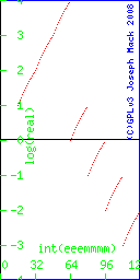 |
The plot is a set of dots (rather than a line or set of lines), showing that you can only represent some of the real space; a few points on the infinity of points that is a line.
| Note |
|---|---|
| End Lesson 18 | |
The representation of the +ve reals is
1..2 * 2^exponent. |
The 8-bit real numbers (from 0.25 to 4.0) on a straight line look like this (because of crowding, reals<0.25 aren't represented)
Figure 2. graph of the 8-bit real numbers from 0.25..4 plotted on a linear real number line.
 |
There are 16 evenly spaced 8-bit real numbers in any 2:1 section of the real number line (e.g. from 0.25..0.50, 0.50..1.0, 1.0..2.0, 2.0..4.0). Because the length of each segment decreases by half each step going leftward (towards 0.0), the real numbers never get to 0.0 (0.0 would be 2-∞).
Logarithms:
If you don't know about logarithms
Logarithms are the exponents when reals are represented as baseexponent.
Logarithms do for multiplication, what linear plots do for arithmetic.
Let's say you want a graph or plot to show the whole range of 8-bit reals from 0.125=2-3 to 16=24. On a linear plot most of the points would be scrunched up at the left end of the line (as happens above). If instead you converted each number to 2x and plotted x, then the line would extend from -3 to +4, with all points being clearly separated.
If n=2x, then x is log2(n). So log2(1)=0, log2(2)=1, log2(4)=2.
If n=20.5, then n2=20.5*20.5=2. Then n=sqrt(2) and 20.5 is sqrt(2).
If you multiply two numbers, you add their logarithms.
Logarithms commonly use base 10 (science and engineering; the log of 100 is 2), base 2 (for computing), and loge (for mathematics, e=2.718281828459)
The 8-bit real numbers (from 0.25 to 4.0) on a logarithmic line look like this
Figure 3. graph of the 8-bit real numbers from 0.25..4 plotted on a log real number line.
 |
Note there are 16 logarithmically spaced real numbers in any 2:1 section of the real number line (e.g. from log2(number) =-2..-1, -1..0, 0..1, 1..2. Because 0.0 is 2-∞, 0.0 on this graph is off the left end of the line (at -∞).
How many real numbers can be represented by a 32 bit number [159] ? How many floating point numbers exist in the range covered by 32-bit reals [160] ?
You can make real numbers as big as you have bits to represent them and as small as you have bits to represent them. However you can't represent 0.0 on the simple floating point scheme shown here.
- We already said that we were going to only represent normalised numbers (which start with the digit 1).
- In the linear plot above, you don't get to 0.0 because the absolute size of each 2:1 range of reals halves at each step as you approach 0.0. In the log plot, 0.0 is at -∞.
However 0.0 is a useful real number. Time starts at 0.0; the displacement of a bar from it's equilibrium position is 0.0.
In the above images/graphs, there is no way to represent 0.0 - it's not part of the scheme. Since a normalised decimal number starts with 1..9 and normalised binary numbers start with 1, how do you represent 0.0? You can't. You need some ad hoc'ery (Ad hoc. http://www.wikipedia.org/wiki/Ad_hoc).
To represent 0.0, you have to make an exception like "all numbers must start with 1-910 or 12, unless it's 0.0, in which case it starts with 0". Designers of rational systems are dismayed when they need ad hoc rules to make their scheme work. ad hoc rules indicate that maybe the scheme isn't quite as good as they'd hoped. Exceptions slow down the computer, as rather than starting calculating straight away, the computer first has to look up a set of exceptions (using a conditional statement) and figure out which execution path to follow.
How do we represent 0.0? Notice that the bits for the exponent in the previous section can be 100 or 000; both represent 1 (20 or 2-0). 8 of our exponents are duplicates. We could handle the duplication, by having the algorithm add 1 to the exponent if it starts with 1, giving us an extra 8 numbers (numbers that are smaller by a factor of 2). However since we don't yet have the number 0.0 anywhere, the convention (in this case of a 1 byte floating point number) is to have two of the 8 numbers with the exponent bits=000 as +/- 0.0. As well we need to represent +/-∞ and NaN, so we use some of the remaining 6 numbers for those.
S see mmmm 0 000 0000 +0.0 1 000 0000 -0.0 (yes there is -0.0) 0 111 0000 +infinity 1 111 0000 -infinity * 111 !0000 NaN |
NaN (not a number): In the IEEE-754 scheme, infinities and NaN are needed to handle overflow and division by 0. Before the IEEE-754 standard, there was no representation in real number space for ∞ or the result of division by zero or over/underflow. Any operation which produced these results had to be trapped by the operating system and the program would be forced to exit. Often these results came about because the algorithm was exploring a domain of the problem for which there was no solution, with division by zero only indicating that the algorithm needed to explore elsewhere. A user would quite reasonably be greatly aggrieved if their program, which had been running happily for a week, suddenly exited with an irrecoverable error, when all that had happened was that the algorithm had wandered into an area of the problem where their were no solutions. The IEEE-754 scheme allows the results of all real number operations to be represented in real number space, so all math operations produce a valid number (even if it is NaN or ∞) and the algorithm can continue. Flags are set showing whether the result came about through over/underflow or division by 0, allowing code to be written to let the algorithm recover.
NaN is also used when you must record a number, but have no data or the data is invalid: a machine may be down for service or it may not be working. You can't record 0.0 as this would indicate that you received a valid data point of 0.0. Invalid or absent data is a regular occurrence in the real world (unfortunately) and must be handled. You process the NaN value along with all the other valid data; NaN behaves like a number with all arithmetic operations (+-*/; the result of any operation with NaN always being NaN). On a graph, you plot NaN as a blank.
The number -0.0: is needed for consistency. It's all explained in "What every computer scientist should know about floating-point arithmetic" (link above). It's simplest to pretend you never heard of -0.0. Just in case you want to find out how -0.0 works...
>>> 0.0 * -1 -0.0 >>> -0.0 * 1 -0.0 >>> -0.0 * -1 0.0 >>> -(+0.0) -0.0 #required by IEEE754 >>> -(+0) 0 #might have expected this to be -0 >>> -0.0 + 0.0 0.0 >>> -0.0 - 0.0 -0.0 >>> -0.0 + -0.0 -0.0 >>> -0.0 - +0.0 -0.0 >>> -0.0 - -0.0 0.0 >>> 0.0 + -0.0 0.0 >>> 0.0 - +0.0 0.0 >>> 0.0 - -0.0 0.0 >>> i=-0.0 >>> if (i<0.0): ... print "true" ... >>> if (i>0.0): ... print "true" ... >>> if (i==0.0): ... print "true" ... true #(0.0==-0.0) is true in python >>> if (i==-0.0): ... print "true" ... true >>> if (repr(i)=="0.0"): ... print "true" ... >>> if (repr(i)=="-0.0"): ... print "true" ... true |
The result of the test (0.0==-0.0) is not defined in most languages. (As you will find out shortly, you can't compare reals, due to the limited precision of real numbers. You can't do it even for reals that have the exact value 0.0).
How many numbers are sacrificed in the 8bit float point representation used here, and in a 32 bit floating point representation (23bit mantissa, 8 bit exponent, 1 bit sign) to allow representation of 0.0, ∞ and NaN [161] ? What fraction of the numbers is sacrificed in each case [162] ?
| Note |
|---|---|
| (with suggestions from the Python Tutorial: representation error). | |
We've found that only a limited number of real numbers (256 in the case of 8-bit reals, 4G in the case of 32-bit reals) can be represented in a computer. There's another problem: most (almost all) of the reals that have finite representation in decimal (e.g.0.2, 0.6) don't have a finite representation in binary.
Only numbers that evenly divide (i.e. no remainder) powers of the base number (10decimal) can be represented by a finite number of digits in the decimal system. The numbers which evenly divide 10 are 2 and 5. Any number represented by (1/2)n*(1/5)m can be represented by a finite number of digits. Any multiple of these numbers can also be represented by a finite number of digits.
In decimal notation, fractions like 1/10, 3/5, 7/20 have finite represenations
1/10=0.1 3/5=0.6 7/20=0.35 |
In decimal notation, fractions like 1/3, 1/7, 1/11 can't be represented by a finite number of digits.
1/3=0.33333.... 1/7=0.14285714285714285714... |
Do these (decimal) fractions have finite representations as decimal numbers: 1/20, 1/43, 1/50 [163] ?
Here's some numbers with finite represenation in decimal.
#(1/2)^3 1/8=0.125 #3/(2^3) 3/8=0.375 #note 1/80 is the same as 1/8 right shifted by one place. Do you know why? #1/((2^4)*5) 1/80=0.0125 #1/(2*(5^2)) 1/50=0.02 #7/(2*(5^2)) 7/50=0.14 |
Using the above information, give 1/800 in decimal [164]
Divisors which are multiples of other primes (i.e. not 2,5) cannot be represented by a finite number of decimals. Any multiples of these numbers also cannot be represented by a finite number of digits. Here's some numbers which don't have finite represenation in decimal.
#1/(3^2) 1/9=0.11111111111111111111... #1/(3*5) 1/15=0.06666666666666666666... #4/(3*5) 4/15=0.26666666666666666666... |
(the Sexagesimal (base 60) http://en.wikipedia.org/wiki/Sexagesimal numbering system, from the Sumerians of 2000BC, has 3 primes as factors: 2,3,5 and has a finite representation of more numbers than does the decimal or binary system. We use base 60 for hours and minutes and can have a half, third, quarter, fifth, sixth, tenth, twelfth, fifteenth, twentieth... of an hour.)
In binary, only (1/2)n can be represented by a finite number of digits. Fractions like 1/10 can't be prepresented by a finite number of digits in binary: there is no common divider between 10 (or 5) and 2.
# echo "scale=10;obase=2;ibase=10; 1/10" | bc -l .0001100110011001100110011001100110 |
In the binary system, the only number that evenly divides the base (2), is 2. All other divisors (and that's a lot of them) will have to be represented by an infinite series.
Here's some finite binary numbers:
echo "obase=2;ibase=10;1/2" | bc -l .1 echo "obase=2;ibase=10;3/2" | bc -l 1.1 #3/8 is the same as 3/2, except that it's right shifted by two places. echo "obase=2;ibase=10;3/8" | bc -l .011 |
From the above information give the binary representation of 3/32 [165]
Knowing the binary representation of decimal 5, give the binary representation of 5/8 [166]
Here's some numbers that don't have a finite represenation in binary
"obase=2;ibase=10;1/5" | bc -l .0011001100110011001100110011001100110011001100110011001100110011001 #note 1/10 is the same as 1/5 but right shifted by one place #(and filling in the empty spot immediately after the decimal point with a zero). echo "obase=2;ibase=10;1/10" | bc -l .0001100110011001100110011001100110011001100110011001100110011001100 |
with the above information, give the binary representation of 1.6 [167]
Here is 1/25 in binary
echo "obase=2;ibase=10;1/25" | bc -l .0000101000111101011100001010001111010111000010100011110101110000101 |
From this information, what is the binary representatin of 1/100 [168]
Just as 1/3 can't be represented by a finite number of decimal digits, 1/10 can't be represented by a finite number of binary digits. Any math done with 0.1 will be done with a 32-bit truncated representation of 0.1
>>> 0.1 0.10000000000000001 >>> 0.1+0.1+0.1+0.1+0.1+0.1+0.1+0.1+0.1+0.1 0.99999999999999989 >>> 0.1*10 1.0 |
The problem of not being able to represent finite decimal numbers in a finite number of binary digits is independant of the language. Here's an example with awk:
echo "0.1" | awk '{printf "%30.30lf\n", $1}'
0.100000000000000005551115123126
echo "0.1 0.1 0.1 0.1 0.1 0.1 0.1 0.1 0.1 0.1" | awk '{printf "%.30lf\n", $1+$2+$3+$4+$5+$6+$7+$8+$9+$10}'
0.999999999999999888977697537484
|
Do not test if two reals are equal. Even though the two numbers (to however many places you've displayed) appear the same, the computer may tell you that they're different. Instead you should test
abs(your_number - the_computers_number) < some_small_number |
For the real way to do it see Lahey compiler.
Here's an example of how things don't work quite the way you'd expect.
>>> i=0.1
>>> if (i==0.1): #is (i==0.1)?
... print "true"
...
true
>>> j=0
>>> for x in range(0,10):
... j += i
...
>>> j #j should be 1.0, but you loose a 1 in the last place every time you add 0.1
0.99999999999999989
>>> print j #outputs field width of 12 (and will round the number)
1.0
>>> print "%20.12f" %j #print with explicit 12 digits after decimal point
1.000000000000
>>> print "%20.20f" %j #wider field
0.99999999999999988898
>>> print 1.0-j
1.11022302463e-16
>>> if (j==1.0): #is (j==1.0)?
... print "true"
... else:
... print j
...
1.0
|
Is (j==1.0) true? The answer is not yes or no; you aren't going to get a sensible answer. Knowing that, you should never ask such a question. In case you aren't convinced, let's see what might happen if you do.
(About 747s Airliner Takeoff Speeds, Boeing 747 http://www.aerospaceweb.org/aircraft/jetliner/b747/ Boeing 747-400 http://en.wikipedia.org/wiki/Boeing_747-400 http://www.aerospaceweb.org/question/performance/q0088.shtml). About diesel locomotives Electric Diesel Hauling II (http://www.cfr.ro/jf/engleza/0310/tehnic.htm) Steam Ranger Enthusiast Pages (http://www.steamranger.org.au/enthusiast/diesel.htm).
You've written the computer code to automatically load the Boeing 747-400ER cargo planes each night at the FedEx Memphis terminal. You have a terminal with 1500 palettes, each palette weighing 0.1Mg (about 200lbs). The max cargo payload is 139.7Mg.
It's 2am. All the packages have arrived by truck and are now sitting on palettes. Let's start loading cargo.
#! /usr/bin/python palettes_in_terminal=[] #make an empty list for the palettes in the terminal awaiting loading palettes_in_747=[] #make another empty list for the palettes loaded onto the plane number_palettes=1500 weight_palette=0.1 weight_on_plane=0.0 max_weight_on_plane=139.7 #account for palettes in terminal #make a list containing 1500 entries of 0.1 for i in range(0,number_palettes): palettes_in_terminal.append(weight_palette) #load plane #while plane isn't full and there are more palettes to load # take a palette out of the terminal and put it on the plane while ((weight_on_plane != max_weight_on_plane) and (len(palettes_in_terminal) != 0)): #the next line is a train wreck version of this #moved_palette=palettes_in_terminal.pop() #palettes_in_747.append(moved_palette) palettes_in_747.append(palettes_in_terminal.pop()) weight_on_plane += weight_palette #print "weight of cargo aboard %f" % weight_on_plane print "weight on plane %f" % weight_on_plane print "max weight on plane %f" % max_weight_on_plane #------------- |
What's this code doing? Swipe the code and run it. Is the plane safe to fly? How overloaded is it? How did the code allow the plane to become overloaded [169] ?
In an hour (at 3am), the plane, with a crew of 2, weighing 412,775 kg (about 400 tons, or 2-8 diesel locomotives), will be sitting at the end of the runway ready to take off, with its cargo and enough jet fuel (241,140l.) to make it across the country in time for the opening of the destination airport at 6am. (Why do the pilots have to wait till 6am, why couldn't they fly in earlier [170] ?) The pilot will spool up the engines, hold the plane for several seconds to check that the engines are running at full power, then let off the brakes, when the plane will start to roll. After thundering 3km down the runway, about a minute later alarms will alert the pilot that the apparently fully functional plane hasn't reached the lift off speed of 290 km/hr. The plane is too far down the runway to abort takeoff [171]. As far as the pilot knows, there is nothing wrong with the plane, only the speed is low. Is the indicated low speed an error and the the plane is really moving at the expected speed? Should the pilot rotate the plane and attempt lift off? He has only seconds to decide. Assuming the runway is long enough for the plane to eventually reach lift off speed, will it lift off [172] ? You'll read all about it in the papers next morning. In fact the pilot has no options and no decision to make. He was committed when he let the brakes off.
Why aren't there crash barriers at the end of the runway [173] ? There are better solutions for handling an overweight plane (see below).
The airline will blame the software company. The owners of the software business will protest that it was a problem with one of the computers that no-one could possibly have anticipated (there are people that will believe this). The american legal system will step in, the business will declare bankruptcy, the owners will have taken all their money out of the business long ago and have enough money to live very comfortably, the workers will be out of a job, and will find their pension fund unfinanced. The owners of the software business will be sued by the airline and the workers, but since the business is bankrupt, there is no money even if the suit is successful. Only the lawyers and the business owners will come out of this in good financial shape.
No-one would ever write such a piece of software. Even if you could equate reals, you wouldn't have written the code this way. Why not [174] ? Fix the code (you need to change the conditional statement). Here's my fixed version [175] .
While the algorithm I used here is completely stupid, the actual method that the FAA uses to calculate the take-off weight of a passenger plane is more stupid (and I'm not making this up): the airline just makes up a value. They guess how much the passengers weigh (and from watching how my luggage is handled at check in, they guess the weight of the baggage). The final decision is left to the pilots (at least in the case of US AirWays 5481 below), who have to decide by looking at the baggage and the passengers, whether it's safe to take off. This is the method that's used in the US. If you were a pilot, could you estimate the weight of passengers to 1% by looking out the cockpit door, down the aisles at the passengers? Pilots are trained to fly planes not to weigh passengers: scales are used to weigh planes.
Considering the consequences of attempting to take off overweight, it would be easy enough to weigh a plane before take-off, as is done for a truck or train: see Weigh Bridge (http://en.wikipedia.org/wiki/Weigh_bridge). Accuracy of current equipment is enough for the job: see Dynamass (www.pandrol.co.za/pdf/weigh_bridges.pdf) which can weigh a train moving at 35kph to 0.3% accuracy.
Planes attempt to take off overweight all the time.
The plane piloted by 7 yr old Jessica Dubroff, attempting to be the youngest girl to fly across the USA, crashed shortly after take off from Cheyenne (see Jessica Dubroff. http://en.wikipedia.org/wiki/Jessica_Dubroff). The plane was overloaded and attempted to take off in bad weather.
Most plane crashes due to overloading occur because the weight is not distributed correctly.
Air Midwest #5841 (http://en.wikipedia.org/wiki/US_Airways_Express_Flight_5481) out of Charlotte NC in Jan 2003 crashed on take off, because (among other things) the plane was overloaded by 600lbs, with the center of gravity 5% behind the allowable limit. The take-off weight was an estimate only, using the incorrect (but FAA approved) average passenger weight estimate, that hasn't been revised since 1936. The supersized passengers of the new millenium are porkers, weighing 20lbs more. The airline washed their hands of responsibility and left it to the pilots to decide whether to take off. Once in the air, the plane was tail heavy and the pilots couldn't get the nose down. The plane kept climbing till it stalled and crashed.
An Emirates plane taking off from Melbourne (http://www.smh.com.au/travel/takeoff-error-disaster-averted-20090430-aozu.html) with 257 passengers, weighed 100tonnes more than the pilots had been told. The Airbus A340-500 scraped its tail along the tarmac and grassland beyond the runway at Tullamarine on March 20, then hit airport landing lights and disabled a radio antenna before taking off. The pilots then dumped fuel over Port Phillip Bay for about 30 minutes to reduce the weight before making an emergency landing at Tullamarine.
One would think that 32-bits is enough precision for a real, and in many cases (just adding or multiplying a couple of numbers) it is. However most of the time spent on computers is optimising multi-parameter models. Much scientific and engineering computing is devoted to modelling (making a mathematical representation for testing - weather, manufactured parts, bridges, electrical networks). You are often optimising a result with respect to a whole lot of parameters; e.g.
- In the scientific world you might be finding a set of parameters which best fit data.
- In business/industry, you might be finding the minimum cost for making a product, by running simulations changing the size or quality of ingredients, the location of the plant(s) making it, the cost of making it, changing various suppliers, the public's likely reaction to a better built (but more expensive) device.
- You might try to optimise making cookies (biscuits outside USA). Your constraints are that the average cookie must have 10 chocolate chips, or 10 raisins, and you need to minimise the cost of ingredients, labour and heat for cooking. As in many optimisations, you can't program in all parameters and you find that the computer optimised result is unusable. In this case your cookies may have an unacceptable taste or texture. Next time you ask the computer for all recipes that will have a total cost below a certain level. You find that the cost is too high to make any money, so you decide to become a computer programmer instead.
Optimisation is similar an ant's method for finding the top of a hill. All the ant knows is its position and it's altitude. It moves in some direction and takes note of whether it has gone uphill or downhill. When it can no longer move and gain altitude, the ant concludes that it is at the top of the hill and has finished its work. The area around the optimum is relatively flat and the ant may travel a long way in the x,y direction (or whatever the parameters are), before arriving at the optimum. Successful optimisation relies on the ant being able to discern a slope in the hill.
Because of the coarseness of floating point numbers, the hill instead of being smooth, is a series of slabs (with consecutive slabs of different thickness). An ant standing next to the edge of a slab, sees no change in altitude if it moves away from the edge, but if it had moved towards the edge would have seen a large change in altitude. If the precision of your computer's floating point calculations is too coarse, the computer will not find the optimum. In computerese - your computation will not converge to the correct answer and you won't be able to tell that you've got the wrong solution, or it will not converge at all - the ant will wander around a flat slab on the side of the hill, never realising that it's not at the top.
If the computation changes from 32 to 64-bit, how many slabs will now be in the interval originally covered by a 32-bit slab [176] ?
Because you can't rely on a 32-bit computation converging or getting the correct answer, scientists and engineers have been using 64-bit (or greater) computers for modelling and optimisation for the past 30yrs. You should not use 32 bit floating point for any work that involves repetitive calculation of small differences.
How do you know that your answer is correct and not an artefact of the low precision computations you're using? The only sure way of doing this is to go to the next highest precision and see if you get the same answer. This solution may require recoding the problem, or using hardware with more precision (which is likely unavailable, you'll already be using the most expensive computer you can afford). Programmers test their algorithm with test data for which they have known answers. If you make small changes in the data, you should get small changes in the answers from the computer. If the answers leap around, you know that the algorithm did not converge.
Money (e.g. $10.50) in a bank account looks like a real, but there is no such thing as 0.1c. Money needs to be represented accurately in a computer in multiples of 1c. For this computers use binary coded decimal (http://en.wikipedia.org/wiki/Binary-coded_decimal). This is an integer representation, based on 1c. You can learn about on this your own if you need it.
| Note |
|---|---|
| End Lesson 19 | |
FIXME. This has not been presented to the students and has several problems. I'll come back to this later.
The smallest number representable by a 64-bit real is 2.2250738585072020*10-308. Its value is mainly limited by the number of digits you can store in the exponent (multiplied by a normalised mantissa whose value has the range 1.0 .. 1.111).
Another small number of interest to computer programmers is the value of the smallest change you can make to a number (let's say number==1.0). This is determined by the number of bits in the mantissa. If the 23 bit mantissa for 1.0 on a 32 bit machine (being normalised) is 000000000000000000000000, then the smallest change will be to 000000000000000000000001 (only the last bit changes). The number represented by this difference is called the machine's epsilon (http://en.wikipedia.org/wiki/Machine_epsilon). The number is called the "machine's epsilon" because before IEEE 754, every machine had a different way of representing reals, and each machine would have its own epsilon. Now with most machines (and except for specialised embedded machines) being IEEE 754 compliant, the machine's epsilon will be the IEEE 754 epsilon. Let's ask our machine what its epsilon is.
>>> epsilon = 1 #has a simple representation in binary >>> while (epsilon+1>1): ... epsilon = 0.5*epsilon #still has a simple representation in binary ... print epsilon ... 0.5 0.25 0.125 . . 7.1054273576e-15 3.5527136788e-15 1.7763568394e-15 8.881784197e-16 4.4408920985e-16 2.22044604925e-16 1.11022302463e-16 |
If to the computer, 1+epsilon==1, the loop exits. The machine's epsilon for 64-bit IEEE 754 reals is 1.11022302463e-16 (for comparison, the smallest representable real is 2.2250738585072020*10-308). (note: epsilon is a lot bigger than the smallest number representable by the machine's reals. Do you understand the difference between these two numbers?)
What this section is saying is that the computer can't differentiate reals that are more closely spaced than the spacing represented by the last bit in the mantissa.
After shifting x=1/5 one place to the right (in the previous section) to give the result x=1/10, note that the right hand "1" falls off the end and is lost. In the following sequence of calculations (right shift, losing the last 1, then left shift, which will insert a 0, in the place which previously had a 1)
x=0.2 y=x/2 #y=0.1 z=y*2 #z=0.2 |
would the resulting z have the same value as the original x? If you were using fixed point operations, you would get a different value. However a computer uses a mantissa and an exponent to represent a real, so dividing by a power of 2 just changes the exponent and no precision is lost. The mantissa will be unchanged following the above operations, and z would have the same value as x.
>>> x=0.2 >>> y=x/2 >>> z=y*2 >>> print z-x 0.0 |
Taking this example to the extreme...
>>> n_128=2**128 >>> print n_128 340282366920938463463374607431768211456 >>> x=0.1 >>> y=x/n_128 >>> z=y*n_128 >>> print "%30.30g, %30.30g, %30.30g" %(x,y,z) 0.100000000000000005551115123126, 2.93873587705571893305445304302e-40, 0.100000000000000005551115123126 |
What if you did an operation that changed the mantissa (ignoring whether or not the exponent was changed)? We need a number that doesn't have a finite representation in binary.
>>> x=0.1 #x doesn't have a finite represenation in binary >>> n_prime=149.0 #1/n_prime doesn't have finite representation in binary either >>> y=x/n_prime >>> z=y*n_prime >>> print "%30.30g, %30.30g, %30.30g, %30.30g " %(x,y,z,z-x) 0.100000000000000005551115123126, 0.000671140939597315508424735241988, 0.100000000000000005551115123126, 0 |
I would have thought that z and x would be different, but you get back the same number. I puzzled about this, till a co-worker Ed Anderson suggested the following as a method to find out what was going on: try a whole bunch of numbers. In particular, try some irrational numbers, like square roots (irrational numbers cannot be represented by a finite number of digits, in any base system). All square roots, except integers, are irrational (for the range 1..10, only 1,4 and 9 would have rational square roots). So use all the square roots from 1..some_large_number for both x and the divisor/multiplier. Ed's initial test was a 100x100 grid. Here's Ed's code for a 64*64 grid. There is a blank when the numbers are identical, and a letter/number if they were different.
#! /usr/bin/python
# fp_ed.py
# Joseph Mack (C) 2008, GPL v3.
# With suggestions from Ed Anderson
# takes a number, divides it by a 2nd, stores the result, then multiplies the result the 2nd number.
# in a perfect world, the result should be the original answer.
# due to limited precision of computer reals, sometimes a different answer will be returned.
from math import sqrt;
number_that_are_different=0;
end = 100;
for j in range(1,end):
output_string = "" # can't output strings without \n in python and can't supress a blank either
output_string += str('%3d ' %j); #put blank after string
for i in range(1,end):
x = sqrt(i);
y = x/j;
z = y*j;
if (x-z == 0.0):
output_string += " "
else:
#print x-z ;
output_string += "x";
number_that_are_different += 1;
print output_string
print number_that_are_different
#- fp_ed.py -----------------------
|
Here's the output
1 2 3 4 5 6 1 2 3 x2 33 3 w 3 3 4 5 1 2 2 333 w 3 3 6 x2 33 3 w 3 3 7 x w w3 w 3 8 9 w w 10 1 2 2 333 w 3 3 11 x 2 w 3w3w ww w 3w 3 3 12 x2 33 3 w 3 3 13 xx ww w w w w 3w 14 x w w3 w 3 15 x w3w 16 17 w 18 w w 19 x w w ww 20 1 2 2 333 w 3 3 21 w 3 w 3 3 3 3 22 x 2 w 3w3w ww w 3w 3 3 23 x 3 3 3 w www3 24 x2 33 3 w 3 3 25 x x w w w w 26 xx ww w w w w 3w 27 xx w ww w w3 w 28 x w w3 w 3 29 2x 33w w3w 30 x w3w 31 w 32 33 34 w 35 2 3 3 3w 3 36 w w 37 y 2 x 33 w w w 38 x w w ww 39 2 33 3 33 w 40 1 2 2 333 w 3 3 41 x 3 3 3 w w 3 42 w 3 w 3 3 3 3 43 1y 2 x2x 2 w 3 w w 3 ww w 3 w 33 44 x 2 w 3w3w ww w 3w 3 3 45 3 w w 3 3 46 x 3 3 3 w www3 47 2x2 2 w333 w 3 w33 w w 48 x2 33 3 w 3 3 49 0 1 2 w w 3 3 3w 50 x x w w w w 51 2 x 3ww33 w 3 w 52 xx ww w w w w 3w 53 22 3 3 3 3 3 3 54 xx w ww w w3 w 55 y xx w3 3w 3 3 w33 56 x w w3 w 3 57 2 3ww3 w 58 2x 33w w3w 59 2x 33w3 w 60 x w3w 61 w w 62 w 63 |
What if we do the multiplication first
1 2 3 4 5 6 1 2 3 y x x w w 3w 3 3 w w 4 5 2 x 3 3w w ww 3 6 y x x w w 3w 3 3 w w 7 x w w3 3 8 9 x x w 3w w3 3 10 2 x 3 3w w ww 3 11 3 w 3 w w3 12 y x x w w 3w 3 3 w w 13 y x 2 2 3 3w w 3 3 3 w 3 14 x w w3 3 15 x w 3 w 16 17 w3 w3 18 x x w 3w w3 3 19 22 w 3 3w 3w3 3 w3 20 2 x 3 3w w ww 3 21 y 2 x2 3w3 w 3 w 3 3w 3 22 3 w 3 w w3 23 2 2 33 3 3 3 33 24 y x x w w 3w 3 3 w w 25 ww ww w 26 y x 2 2 3 3w w 3 3 3 w 3 27 1 2 2 w w 3 w 3 3 w 3 3 28 x w w3 3 29 w w w3 30 x w 3 w 31 3 3 32 33 w3 34 w3 w3 35 3 3 36 x x w 3w w3 3 37 2 3w3 w 3 38 22 w 3 3w 3w3 3 w3 39 y xx 2 ww3 w w ww3 3 3 40 2 x 3 3w w ww 3 41 x x 3 w 333 w 3 www 42 y 2 x2 3w3 w 3 w 3 3w 3 43 2 3 ww 3 w 3 44 3 w 3 w w3 45 y 2xx w w 3 ww w w 46 2 2 33 3 3 3 33 47 y x 2x w 33 3 3www 3 48 y x x w w 3w 3 3 w w 49 x 3 3 w ww 3w 3 50 ww ww w 51 1 2 22 3 3 33 3 w 52 y x 2 2 3 3w w 3 3 3 w 3 53 2x 33 w 3 3 w 54 1 2 2 w w 3 w 3 3 w 3 3 55 x w w 3 3 w 3 56 x w w3 3 57 3 w 3 w 58 w w w3 59 x 3 w 3 w 60 x w 3 w 61 w 62 3 3 63 3 |
The figures are different. It seems that multiplication and division isn't always commutative.
Surprisingly (to me) there is a pattern, but then I didn't understand what was going on so any result would have been a surprise. "x"s appear in blocks on boundaries which are multiples of 8,16,32 and 64 (increasing the value of end shows that the block pattern continues).
With a slight modification of the code, the differences, if not 0.0, were all seen to be (1.11022302463e-16)*2n.
Is there anything in particular about 1.11022302463e-16? It turns out that it's the machine's epsilon (http://en.wikipedia.org/wiki/Machine_epsilon) (also see machine's epsilon).
What is 1.11022302463e-16 in binary?
dennis:~# echo "obase=2;1.11022302463*10^-16" | bc -l .0000000000000000000000000000000000000000000000000000011111111111111 |
If you round this up by one bit, it's 2^-53. A 64 bit double has a 53 bit mantissa, indicating that the epsilon calculation is using a 64 bit real.
From the wiki entry, a single precision (32bit) real has a 24 bit mantissa. 1.0 then has an exponent of 0 and mantissa of 1.000000000000000000000002. The next biggest number has an exponent of 0 and a mantissa of 1.000000000000000000000012. The difference is 0.000000000000000000000012 or 2-23.
Using IEEE 754 Converter (http://www.h-schmidt.net/FloatApplet/IEEE754.html), to do the conversion to a 32-bit real, I found
1.11022302463e-16=0x2500000=00100101000000000000000000000000. |
Breaking the binary representation into sign, exponent and mantissa (with the implied 1 for a normalised mantissa) gives
1.11022302463e-16 = 0 01001010 (1)00000000000000000000000
decimal s exp mantissa
|
Calculating this all gives: The sign bit: (bit 32, the leftmost bit) is 0 (positive).
The exponent: the IEEE-754 real math convention doesn't use the signed int representation. a 32 bit real, the exponent is a 9 bit integer (here 001001010). Floating point math is usually done on floating point hardware (or emulated on the the integer registers of the CPU, but the incremental cost of adding a floating point processor/unit (FPU) is small, so all x86 chips, starting with the 486, have a floating point processor built-in to the CPU chip). Since real math doesn't use the CPU's registers (each composed of 2,4,8 or 16 bytes), but instead uses the math co-processor's registers, then real math doesn't have to use the CPU's conventions (e.g. a signed int) to process a 9 bit int.
For 32 bit floating point, the convention is to subtract 127 from the value of the exponent. is is called "excess-127" (excess-1023 for 64 bit) and allows the exponent and the mantissa, when taken together, to vary monotonically (see IEEE-754 References http://babbage.cs.qc.edu/courses/cs341/IEEE-754references.html). (What this gets you, I don't know.) The 8-bit scheme 8-bit set of normalised reals I made up for this class is not monotonic in this respect (see the table and the figure, where there are jumps in value every 16 numbers).
In the current example, the exponent is -53 (from the next 9 bits). To get the actual value of the exponent, you subtract 127.
echo "obase=10; ibase=2; 001001010" | bc 74 then subtract 127 74-127=-53 |
The FPU int then is an unsigned int, from which is subtracted 127, so that -ve numbers are possible (it's called signed magnitude). Here are a few comparison numbers (assuming an 8 bit int):
bits value, signed int value, unsigned int value, signed magnitude 00000000 0 0 -127 00000001 1 1 -126 01111111 127 127 0 10000000 -127 128 1 11111111 -1 255 128 |
Since all of the evaluations can done with the same speed, with hardware designed to do these calculations, there is nothing to pick between them. Why IEEE-754 uses their particular representation of the exponent, rather than the signed int representation, I don't know.
The mantissa is 1.0 (after adding the implied 1 at the beginning of 23 zeroes).
Multiplying this all out gives the original number.
echo "1*2^-53" | bc -l .00000000000000011102 #just checking that I can count 0s echo "1*2^-53/10^-16" | bc -l 1.11020000000000000000 |
The following table shows the number of times an entry occured for a grid size. The 2nd entry says that in an 16*16 grid, that 206 numbers were not changed and that -(1.11022302463e-16)*23 was returned 9 times, +(1.11022302463e-16)*2*2 was returned 2 times and that +(1.11022302463e-16)*2*3 was returned 8 times. In the 16*16 grid 15*15=225 numbers are tested (=9+206+2+8).
grid size\n -8 -7 -6 -5 -4 -3 -2 -1 0 1 2 3 4 5 6 7 8 8*8 0 0 0 0 0 0 0 0 0 0 0 0 48 0 1 0 0 0 0 0 0 0 0 0 0 16*16 0 0 0 0 0 0 0 0 0 9 0 0 206 0 2 8 0 0 0 0 0 0 0 0 0 32*32 0 0 0 0 0 0 0 0 6 22 0 0 911 0 3 13 6 0 0 0 0 0 0 0 0 64*64 0 0 0 0 0 0 0 0 163 44 3 0 3566 1 6 33 153 0 0 0 0 0 0 0 0 128*128 0 0 0 0 0 0 0 99 346 82 10 0 15062 4 14 80 349 83 0 0 0 0 0 0 0 256*256 0 0 0 0 0 0 0 3085 723 163 24 0 56990 14 39 174 750 3063 0 0 0 0 0 0 0 512*512 0 0 0 0 0 0 1679 6215 1505 355 56 0 241228 35 87 381 1570 6360 1650 0 0 0 0 0 0 1024*1024 0 0 0 0 0 0 50447 12720 3101 752 121 0 911185 91 196 799 3209 12807 51101 0 0 0 0 0 0 2048*2048 0 0 0 0 0 26941 101676 25687 6251 1500 250 0 3863963 230 452 1669 6449 25610 102498 27033 0 0 0 0 0 4096*4096 0 0 0 0 0 822872 204267 51363 12576 3001 525 0 14575322 504 969 3366 12919 51254 205106 824981 0 0 0 0 0 8192*8192 0 0 0 0 432519 1647991 409597 102641 25183 5958 1057 0 61830620 1105 2100 6885 25992 103109 411309 1652318 434097 0 0 0 0 16384*16384 0 0 0 0 13222697 3300406 821156 205169 50246 11827 2083 0 233145705 2345 4366 13903 52320 206826 824241 3306218 13233181 0 0 0 0 32768*32768 0 0 0 6931293 26447787 6604323 1645180 409899 100085 23405 4099 0 989292832 4872 9022 28195 105323 414810 1651250 6614158 26462945 6926811 0 0 0 65536*65536 0 0 0 211603215 52895451 13214901 3295139 820314 200000 46646 8163 0 3730616481 9841 18209 56688 211726 830962 3306011 13229067 52912230 211561181 0 0 0 131072*131072 262144*262144 524288*524288 1048576*1048576 8*8 0.0 0.0 0.0 0.0 0.0 0.0 0.0 0.0 0.0 0.0 0.0 0.0 0.980 0.0 0.020 0.0 0.0 0.0 0.0 0.0 0.0 0.0 0.0 0.0 0.0 16*16 0.0 0.0 0.0 0.0 0.0 0.0 0.0 0.0 0.0 0.040 0.0 0.0 0.916 0.0 0.009 0.036 0.0 0.0 0.0 0.0 0.0 0.0 0.0 0.0 0.0 32*32 0.0 0.0 0.0 0.0 0.0 0.0 0.0 0.0 0.006 0.023 0.0 0.0 0.948 0.0 0.003 0.014 0.006 0.0 0.0 0.0 0.0 0.0 0.0 0.0 0.0 64*64 0.0 0.0 0.0 0.0 0.0 0.0 0.0 0.0 0.041 0.011 0.001 0.0 0.898 0.0 0.002 0.008 0.039 0.0 0.0 0.0 0.0 0.0 0.0 0.0 0.0 128*128 0.0 0.0 0.0 0.0 0.0 0.0 0.0 0.006 0.021 0.005 0.001 0.0 0.934 0.0 0.001 0.005 0.022 0.005 0.0 0.0 0.0 0.0 0.0 0.0 0.0 512*512 0.0 0.0 0.0 0.0 0.0 0.0 0.006 0.024 0.006 0.001 0.0 0.0 0.924 0.0 0.0 0.001 0.006 0.024 0.006 0.0 0.0 0.0 0.0 0.0 0.0 1024*1024 0.0 0.0 0.0 0.0 0.0 0.0 0.048 0.012 0.003 0.001 0.0 0.0 0.871 0.0 0.0 0.001 0.003 0.012 0.049 0.0 0.0 0.0 0.0 0.0 0.0 2048*2048 0.0 0.0 0.0 0.0 0.0 0.006 0.024 0.006 0.001 0.0 0.0 0.0 0.922 0.0 0.0 0.0 0.002 0.006 0.024 0.006 0.0 0.0 0.0 0.0 0.0 4096*4096 0.0 0.0 0.0 0.0 0.0 0.049 0.012 0.003 0.001 0.0 0.0 0.0 0.869 0.0 0.0 0.0 0.001 0.003 0.012 0.049 0.0 0.0 0.0 0.0 0.0 8192*8192 0.0 0.0 0.0 0.0 0.006 0.025 0.006 0.002 0.0 0.0 0.0 0.0 0.922 0.0 0.0 0.0 0.0 0.002 0.006 0.025 0.006 0.0 0.0 0.0 0.0 16384*16384 0.0 0.0 0.0 0.0 0.049 0.012 0.003 0.001 0.0 0.0 0.0 0.0 0.869 0.0 0.0 0.0 0.0 0.001 0.003 0.012 0.049 0.0 0.0 0.0 0.0 32768*32768 0.0 0.0 0.0 0.006 0.025 0.006 0.002 0.0 0.0 0.0 0.0 0.0 0.921 0.0 0.0 0.0 0.0 0.0 0.002 0.006 0.025 0.006 0.0 0.0 0.0 65536*65536 0.0 0.0 0.0 0.049 0.012 0.003 0.001 0.0 0.0 0.0 0.0 0.0 0.869 0.0 0.0 0.0 0.0 0.0 0.001 0.003 0.012 0.049 0.0 0.0 0.0 131072*131072 262144*262144 524288*524288 1048576*1048576 |
After the multiplication/division, how many numbers are returned with a different value? For any particular j you have a 50% chance of losing a 0 off the right end, in which case you'll get back the original answer. So one possibility is 50% will be different. How about the divisor?; you only have a 50% chance of getting that right when you drop off extra digits. With two ways of getting it wrong, you only have 25% chance of getting it right, so 75% will be different. Here's the results.
grid_size number_mul/div number_changed %changed largest_difference 10*10 10^2 2 2 + 4 * 1.11e-16 100*100 10^4 713 7 +- 16 * 1.11e-16 1000*1000 10^6 127980 13 +- 32 * 1.11e-16 10000*10000 10^8 8060303 8 +- 128 * 1.11e-16 100000*100000 10^10 927798399 9 +- 512 * 1.11e-16 |
Let's look at this example with the IEEE-754 converter referred to above
>>> sqrt(14) 3.7416573867739413 >>> x=sqrt(14) >>> y=x/3 >>> z=y*3 >>> z-x -4.4408920985006262e-16 |
#from IEEE 754 converter x = 3.7416573867739413 = 2 * 1.8708287 = 0 10000000 (1) 11011110111011101010001 3.0 = 2 * 1.5 = 0 10000000 (1) 10000000000000000000000 #from python y = x/3.0 = 1.247219128924647 = 0 01111111 (1) 00111111010010011100000 #from bc echo "obase=10;ibase=2; 1.11011110111011101010001/1.10000000000000000000000" | bc -l 1.24721916516621907552 echo "obase=2;ibase=2; 1.11011110111011101010001/1.10000000000000000000000" | bc -l 1.0011111101001001110000010101010101010101010101010101010101010101010 #from python z = 3.7416573867739409 from bc echo "obase=10;ibase=2; 1.0011111101001001110000010101010101010101010101010101010101010101010 *11" | bc -l 3.7416574954986572265489474728439311945749068399891257286071777343750 echo "obase=2;ibase=2; 1.0011111101001001110000010101010101010101010101010101010101010101010 *11" | bc -l 11.101111011101110101000011111111111111111111111111111111111111111111 The result after right shifting by one (to give an exponent of 1), and dropping the implied leading 1 from the mantissa give a mantissa of 11011110111011101010000 #new mantissa (after dropping extra digits) 11011110111011101010001 #original mantissa 1 #difference since the exponent is 1 (a factor of 2) then the difference is |
In the following sections we're going to code up two algorithms.
The first, the square root, converges quickly, but like most quickly converging algorithms, can't be generalised to any other calculation: it only works for square roots. The computing landscape is sparsely populated with these quickly converging algorithms and the discovery of such algorithms are isolated events requiring the efforts or inspiration of some genius. Understanding these algorithms doesn't give you any help discovering new algorithms, but some people turn out to be better producing new algorithms than others, and these people understand all the known algorithms. Computer programmers spend a much effort looking for fast algorithms and the discovery and the discoverers are celebrated in the same way as the discovery of new continent is celebrated by the general populace.
One of the better known algorithm people is Donald Knuth (http://en.wikipedia.org/wiki/Donald_Knuth), who is famous for offering cash rewards ($2.56, a hexadecimal dollar according to Knuth) for finding mistakes in his code. Finding a mistake by Knuth is so rare that Knuth's checks (cheques) are one of computerdom's most prized trophies. People prefer to prominently display Knuth's check (cheque) on their wall for the gasps and admiration of vistors, than to deposit the money in their bank account.
Knuth is one of the people who have pushed the concept of mathematically provably correct code. While it's obvious to everyone that a plane manufacturer must show that their plane will fly, the equivalent proof of usability in computing is difficult to demonstrate. Computer code has sufficient traps, bugs and unpredictable responses to out of bounds input, that in the absence of tools to show that code does exactly what it's supposed to do and nothing else, computer programmers rarely attempt to prove that their code is correct. (One of the diagnostic features of computer programs is that they don't work well.) It seems that proving code correct is not generally possible. Knuth once said "Beware of bugs in the above code; I have only proved it correct, not tried it." Computer programmers have given up on provably correct code and currently have adopted the less rigourous, but hopefully achievable goal of of Programming by Contract (http://en.wikipedia.org/wiki/Design_by_contract). Programming by contract is used in Eiffel and Ada (and less so in C++). In languages which don't have Programming by Contract features, programmers are encouraged to put in equivalent statements (even if only in comments) in their code. The built in Programming by Contract features of Ada make it the language of choice for applications where safety is paramount (e.g. Air Traffic Control).
The discovery of the Fast Fourier Transform (http://en.wikipedia.org/wiki/Fast_Fourier_transform) (FFT) and the Monte Carlo Method (http://en.wikipedia.org/wiki/Monte_Carlo_method), both of which came out of people who worked on the Manhattan project, have revolutionised signal processing and statistics respectively, creating whole industries which would not have been possible otherwise.
The second algorithm, which calculates the value of π, uses an easy to understand and generalisable method: numerical integration. Numerical integration is a brute force method that converges so slowly that it is only usable for a small number of significant figures. Often this is enough for computing purposes (you have to accept the long time, whether you like it or not). If you're doing a calculation for which no-one has discovered a quickly converging algorithm, numerical integration will often be your only choice. While in principle you could do a few square roots by hand, numerical integration, being a brute force method, requires computers (or supercomputers) to be usable at all.
Square roots are often used in computer to calculate distances (from Pythagorus). In graphics (e.g. gaming) the inverse square root is used to normalise 3-D vectors (i.e. make sure that between the r,g,b channels, you aren't outputting more than 1 unit of light). Unlike the distance calculation, the inverse sqrt() doesn't have to be all that accurate. There is a fast inverse sqrt() for graphics, see Origin of Quake3's fast inverse square root (http://www.beyond3d.com/content/articles/8/).
There are manuscripts from 1650BC referring to Egyptian methods of extracting square roots (see wiki square root. http://en.wikipedia.org/wiki/Square_root#History).
There is a sqrt() in the python math module. It calls the C math libraries, which call the hardware sqrt() function on your computer's floating point unit (fpu). The sqrt() then is being done in special hardware. You aren't going to get any faster than that. Despite the ready availability of a fast accurate sqrt(), we're going to use one of the simpler sqrt() methods, the Babylonian method, an algorithm well suited to hand calculation.
First we need to know the precision (number of significant figures) that python uses to represent real numbers. (What is the precision for integers [177] ?) Remember that a 32 bit computer can manipulate 232 integers (you do remember the value of 232? - it's about 10 decimal digits). We'll learn more about Real Numbers later, but for the moment we won't go far wrong if we assume that a 32 bit computer is capable of representing 232 real numbers. While there is only one integer between 0..2, there can be an infinite number of reals 0..2 and a computer can't hope to represent all of them. The computer finds the nearest one it can represent, whether it's correct or not, and say "it's near enough". If we go to 64-bits, we'll get a more accurate representation, but it still won't be exact.
Here's some code to show that floating point numbers longer than 12 digits are truncated i.e. any following numbers are garbage.
>>> for x in range (1,15): ... print x, 1+10**-x ... 1 1.1 2 1.01 3 1.001 4 1.0001 5 1.00001 6 1.000001 7 1.0000001 8 1.00000001 9 1.000000001 10 1.0000000001 11 1.00000000001 12 1.0 13 1.0 14 1.0 |
1012 is 2? [178] This is not enough accuracy for a 64 bit number and is too much for a 32 bit number. We should suspect that we've goofed. The above truncation turns out to be due to limitations of the formatting. print uses str() for outputting, which only outputs 12 digits after the decimal point. If we increase the number of digits displayed, you can get about 15 significant figures before getting garbage. (Note: we are finding the machine's epsilon).
>>> for x in range (1,20): ... print "%2d, %10.40f" %( x, 1+10**-x) ... 1, 1.1000000000000000888178419700125232338905 2, 1.0100000000000000088817841970012523233891 3, 1.0009999999999998898658759571844711899757 4, 1.0000999999999999889865875957184471189976 5, 1.0000100000000000655120402370812371373177 6, 1.0000009999999999177333620536956004798412 7, 1.0000001000000000583867176828789524734020 8, 1.0000000099999999392252902907785028219223 9, 1.0000000010000000827403709990903735160828 10, 1.0000000001000000082740370999090373516083 11, 1.0000000000100000008274037099909037351608 12, 1.0000000000010000889005823410116136074066 13, 1.0000000000000999200722162640886381268501 14, 1.0000000000000099920072216264088638126850 15, 1.0000000000000011102230246251565404236317 16, 1.0000000000000000000000000000000000000000 17, 1.0000000000000000000000000000000000000000 18, 1.0000000000000000000000000000000000000000 19, 1.0000000000000000000000000000000000000000 |
of course we hoping to get
1, 1.1000000000000000000000000000000000000000 2, 1.0100000000000000000000000000000000000000 3, 1.0010000000000000000000000000000000000000 4, 1.0001000000000000000000000000000000000000 5, 1.0000100000000000000000000000000000000000 6, 1.0000010000000000000000000000000000000000 7, 1.0000001000000000000000000000000000000000 8, 1.0000000100000000000000000000000000000000 9, 1.0000000010000000000000000000000000000000 10, 1.0000000001000000000000000000000000000000 11, 1.0000000000100000000000000000000000000000 12, 1.0000000000010000000000000000000000000000 13, 1.0000000000001000000000000000000000000000 14, 1.0000000000000100000000000000000000000000 15, 1.0000000000000010000000000000000000000000 16, 1.0000000000000001000000000000000000000000 17, 1.0000000000000000100000000000000000000000 18, 1.0000000000000000010000000000000000000000 19, 1.0000000000000000001000000000000000000000 |
Any calculation of reals using python, will only be accurate to about the 15th place. 15 decimal places requires 50 bits (here "l" is log)
# echo "15*l(10)/l(2)" | bc -l 49.82892142331043521840 |
The IEEE double precision (64 bit) representation of real numbers uses 52 bits (close enough to the 50 bits we see above) to represent the mantissa, 11 bits for the exponent and 1 bit for the sign - see IEEE 754-1985 (http://en.wikipedia.org/wiki/IEEE_floating_point_standard#Double-precision_64_bit). It looks like python is using double precision (64 bit) to represent real numbers.
You start with your number>1, and an estimate of the square root (Many algorithms require you to give it starting value(s). Often these can be almost anything.) The square root is going to be somewhere between the number and 1, so make the estimate the arithmetic mean (the average).
estimate = (number + 1.0)/2.0 |
You use this estimate to get a better estimate
new_estimate = (estimate + number/estimate)/2.0 |
How does this work? Let's find the square root of 9.
number = 9 estimate = (9+1)/2.0=5.0 new_estimate = (5 + 9/5))/2.0 = 3.4 |
We started with estimate=5.0 and get estimate=3.4, which is closer to the answer. The estimate gets closer to the known answer with each iteration (the algorithm is said to converge). When we eventually get to our answer (at least within the precision of a real), there will be no change when we plug in the estimate.
estimate = 3 new_estimate = (3 + 9/3))/2.0 = 3 |
We keep iterating till the difference between the estimate and then new_estimate is acceptable. (for the proper way to do real comparisons see Lahey compiler) We could use division to test if they are close enough; this will be slow, but will work no matter what size the number is. We could use substraction, which is fast, but the remainder will be large for large numbers and small for small numbers. Ideally we'd like to get the maximum precision possible (double precision), but for the exercise, we'll substract and use a relatively large difference to terminate the algorithm.
Before we write the code that iterates, we need to initialise some numbers
- the value of the difference which we'll use to detect convergeance. Call it "error" and give it a value of 10-12
- the number for which we need the square root (let's start with 9 and call it "number")
- an estimate of the square root (call it "estimate")
- a better estimate of the square root, based on the first estimate (call it "new_estimate").
Write some code that does these 4 steps and prints out the value of number and the estimate. Here's my code [179] .
We are about to enter a loop. We don't know how many iterations are going to be needed, but we do have a test to show that we're done. Should we use a for loop or a while loop [180] ?
At the top of the while loop we test if we should enter the loop again. What's the test that we've found the square root and how do we use it in the while line? Here's my code [181]
Assume that the loop is entered (i.e. we don't have the square root yet): Before you entered the loop, when you initialised a few variables, you generated an estimate of the square root and from it a better estimate. You should use exactly the same steps to inside the while loop, to generate a better value of estimate. Heres what happens inside the loop:
- You have two estimates for the square root: estimate and a better one new_estimate. Now that you're in the loop, you don't need the current value of estimate any more. You should update its value (with what?).
- You've also decided that new_estimate is not good enough (the test for entering the loop showed it to be too different from estimate). You should get a better value for new_estimate.
Write code to do this, and inside the loop, print out the value for estimate. Here's my code [182] .
| Note |
|---|---|
In a for loop, the code for the calculations is all inside the loop. In a while loop, the code for the calculations must also be ahead of the loop (where it runs once), so that the first time the conditional test in the while statement is run, all values will be known. | |
Where to have the print() statement: For the final code the print() statement will be commented out, so this decision isn't all that important. You can print out values at any step in the while loop and everyone reading your code will know what you've done. The location given is slightly better, as you're printing out the value that caused the loop to be executed. After the loop exits, the last value of new_estimate will be printed by a statement in the following code. If you'd printed after the calculation of new_estimate, then the value for the first iteration of the loop would not be printed.
The only modification left is to print out the final value for the square root [183] .
The order of an algorithm e.g. O(n), O(nlogn) describes the rate at which algorithm's execution time increases with the amount of data that it processes. The calculation of the square root has no data (that can be varied), so we can't use this measure. Instead the measure of worth is the increase in running time needed to increase accuracy by one decimal digit (i.e. a factor of 10).
With a print() statement in the loop, you can see the number of iterations before the answer converges (arrives within the acceptable limit).
On Paul Hsieh's Square Root page (http://www.azillionmonkeys.com/qed/sqroot.html) you'll find that you only need 6 iterations to get 53 places in a 64 bit double precision real number, i.e. every iteration gets you 9 bits, a factor of 29=512, closer to your answer. This is pretty fast.
| Note |
|---|---|
| End Lesson 20 | |
At this stage we have working code for the Babylonian sqrt(). The algorithm converges quickly (only 6 iterations are required to calculate to an accuracy of 53 bits). However saying that it "converges quickly" doesn't quantify anything (it's a phrase from marketing). You need to be able to say how quickly, using a measurement that is meaningful to just about anybody (e.g. your grandma), not just computer programmers. An obvious first test is to compare the Babylonian sqrt() to the best sqrt() you have (the math module sqrt()). If it's better, we'll do more tests, otherwise we'll just drop it.
To do speed tests on code, we need to be able to measure the execution time of a program. Python has a timer that measures wall clock time in seconds since 1 Jan 1970 (the start of unix time). (see Time access and conversions http://docs.python.org/lib/module-time.html). time() is a (apparently 32-bit) float. On some systems the resolution is only 1sec (programs that run for less than 1 sec will appear to run for 0 time). If the computer is otherwise idle, the wall clock time and the execution time of your program are nearly the same. Here's some code to measure time.
from time import time n = 1000000 start = time() #do something n times finish = time() print "execution time per iteration = %10.10f", (finish-start)/n |
A single calculation of a square root is a little fast for most timers. We usually do a large number of iterations in a loop and then divide by the number of iterations. This brings its own problems: we have to figure out how much time is taken up by the looping code, but we can handle that too (see below). To time your square root code, first make your Babylonian sqrt() into a function. Copy your Babylonian sqrt code to a new file square_root_compare.py
- name the function babylonian_sqrt(), giving it one parameter (my_number).
- comment out the line "number = 9" (since the value of number will now come from the parameter) and change all instances of "number" to "my_number".
- comment out the print functions (so it will run faster).
- return new_estimate.
You now have a function. From here on, this function is just a block of code, that you'll do timing runs on. You won't be changing anything inside of it; it's just a black box.
You need a main() to call the function. Write a two-line main() to test your function - assign the variable number the value 1000, and then call babylonian_sqrt() with the parameter number. Test that your code runs.
To do timing runs on the function, main() needs to generate a whole lot different numbers to feed to your the function. Why don't you just feed the same number over and over? Compilers and interpreters are supposed to be smart. If they see you do the same operation over and over on the same data, the compiler/interpreter will recognise what's going on and will just return the same answer, without going through the bother of calculating it over and over. You don't know if your python interpreter is this smart (how would you find out [184] ), but you should expect that one day you'll bump into a smart compiler/interpreter, and your timing runs will be meaningless. You may as well start writing your benchmarking code correctly from the start.
One way of producing a whole lot of different numbers is to use all the numbers produced by range(1,largest_number), where largest_number is say 10,000.
- create a variable largest_number to be the number of times you'll call your function. Give it a value of 10000.
- write a loop to create a number (call it number) that with each iteration assumes the next value from the list 1..largest_number. Do you use a for or a while loop [185] ?
- inside the loop, call babylonian_sqrt() with number as a parameter.
You now have a block of code in main() that calls the function largest_number of times. You now want to time that block
- use an import statement to import the function time() from the module time (confusing huh).
- write code that assigns times to the variables start and finish immediately before the block and immediately after it.
-
Use the values of largest_number, start, finish to print out a line saying
largest number 1000 time/iteration 0.0000341
Here's my code [186] . This outputs the time required to calculate the square roots of all the numbers in the range 1..1000. This piece of timing code is a self contained block. You aren't going to change it (except for the value of largest_number)
The average time for the sqrt() calculation depends on the number of times you looped (it shouldn't, but it does). You'll find that the time/iteration depends on whether you did it 10,100 or 1,000,000 times. You need to find a range of largest_number for which the time/iteration is the fastest availalbe and relatively constant. To handle this, you need to call the timing loop with a range of values of largest_number. To do this, put the timing loop above, inside another loop, which feeds different values of largest_number into the timing loop. Putting one loop inside another is called "nesting loops".
To do this, you'll need to use a list. Go to the section explaining lists and then return here.
Create a list named largest_numbers[] holding the values 1,10,100....1000000. Read these values out, using a loop (for or while?) assigning the values one at a time to largest_number. The timing loop, being nested inside the new outer loop, will now have to be indented one step to allow it to be parsed correctly. Here's what the nested loops look like
largest_numbers=[1,10,100,1000,10000,100000,1000000] #list of values for outer loop for largest_number in largest_numbers: #new outer loop for number in range(0,largest_number): #original loop babylonian_sqrt(number) |
Here's my code [187] .
Here's my output
# ./square_root_compare.py largest number 1 time/iteration 0.0001909 largest number 10 time/iteration 0.0000348 largest number 100 time/iteration 0.0000295 largest number 1000 time/iteration 0.0000341 largest number 10000 time/iteration 0.0000398 largest number 100000 time/iteration 0.0000474 largest number 1000000 time/iteration 0.0000512 |
Look to see if there's a range of values for largest_number where time for doing a sqrt is independant of the loop size (it should be the fastest time). For largest_number having a value of 10 or more, the Babylonian square root function takes 30-50usec on my 1GHz machine. One one student's machine (MacOS), the time/interation kept dropping with in the range values for largest_number above, so I sent him off to do runs with increasing values of largest_number. Another student's machine (WinXP) reported 0 time for the first 3 runs, and presumably has a time() function with a resolution of only 1 sec.
| Note |
|---|---|
| End Lesson 21 | |
Next we want to compare the speed of the Babylonian sqrt() to the built-in sqrt() (in the math module).
- Add another timing loop for the built-in sqrt() at the same level as the timing loop for the babylonian_sqrt(). Add an extra section to the outer loop in main() which calls sqrt() from the math module.
- add timers to this new block to measure the execution time of the built-in sqrt(). you can reuse the names start, finish since the babylonian_sqrt() timing loop has exited and is not using these variables anymore.
- add a print line to output the times.
Here's the new calling code in main() [188] .
Calling range() and setting up the looping consumes cpu cycles, so we need to subtract that time from our results. Code up a 3rd timing loop that doesn't do anything, so later you can subtract that time out. Here's a loop that does nothing (you can't have an empty line, the parser gets confused).
for number in range(0,largest_number): pass |
Here's my code [189] . Here's the output
# ./square_root_compare.py babylonian_sqrt: largest number 1 time/iteration 0.0001969337 library_sqrt: largest number 1 time/iteration 0.0000259876 empty_loop: largest number 1 time/iteration 0.0000119209 babylonian_sqrt: largest number 10 time/iteration 0.0000346184 library_sqrt: largest number 10 time/iteration 0.0000043154 empty_loop: largest number 10 time/iteration 0.0000017881 babylonian_sqrt: largest number 100 time/iteration 0.0000295210 library_sqrt: largest number 100 time/iteration 0.0000031996 empty_loop: largest number 100 time/iteration 0.0000008512 babylonian_sqrt: largest number 1000 time/iteration 0.0000341501 library_sqrt: largest number 1000 time/iteration 0.0000030880 empty_loop: largest number 1000 time/iteration 0.0000007720 babylonian_sqrt: largest number 10000 time/iteration 0.0000398650 library_sqrt: largest number 10000 time/iteration 0.0000031442 empty_loop: largest number 10000 time/iteration 0.0000007799 babylonian_sqrt: largest number 100000 time/iteration 0.0000459829 library_sqrt: largest number 100000 time/iteration 0.0000033149 empty_loop: largest number 100000 time/iteration 0.0000009894 babylonian_sqrt: largest number 1000000 time/iteration 0.0000511363 library_sqrt: largest number 1000000 time/iteration 0.0000033719 empty_loop: largest number 1000000 time/iteration 0.0000010112 |
The time for the empty loop is 0.7-1.0usec. Here's the timing results, after subtracting the empty loop time.
Table 2. square root (time, usec): Babylonian and math library code
| Babylonian | math library |
|---|---|
| 30-50 | 2 |
The library sqrt() is 15-25 times faster than the Babylonian sqrt(). Even though the babylonian_sqrt() only needs 5 iterations to get the answer, the library routine gets the answer in the time of 1/3-1/5th of a loop.
Python being an interpretted language will be slower than a compiled language. As well, python is object oriented, making it slower yet. C is one of the languages of choice when speed is required. Here's the same program as above (comparing the Babylonian and math library sqrt()) written in C (it uses the low resolution timers). With your current programming knowledge, you should be able to read this code and know what it's doing. [190] . Here's the output
time/iteration: babylonian 10000000 0.00000122000000000000 time/iteration: library 10000000 0.00000010800000000000 time/iteration: empty 10000000 0.00000000700000000000 time/iteration: babylonian 100000000 0.00000135340000000000 time/iteration: library 100000000 0.00000010790000000000 time/iteration: empty 100000000 0.00000000680000000000 time/iteration: babylonian 1000000000 0.00000147792000000000 time/iteration: library 1000000000 0.00000010824000000000 time/iteration: empty 1000000000 0.00000000691000000000 |
Here's the comparison of the timing results, subtracting 7nsec for the empty loop (compared to 700nsec for the empty loop in python).
Table 3. square root (time, usec): Babylonian and math library code
| Language | Babylonian | math library |
|---|---|---|
| python | 30-50 | 2 |
| C | 1.3 | 0.11 |
| ratio time Python/C | 25-40 | 20 |
C is 20-40 times faster than python, at least for doing sqrt(). So why does anyone code in python? If speed is your main requirement you don't. However it takes longer to write C than it does to write python and people who don't program a lot, can write working python without too much trouble, but may not be able to get a C program to work. If you only require a few square roots and it takes 5 mins to write it in python and 10 mins to write it in C, then you do it in python. If you need to do 1012 square roots, then you do it in C.
If your code only takes 1 min to run and you're only going to run it a couple of times, then you really don't care if it takes 10 times longer. However if you're going to be running the 1 minute program hundreds of times, or your program will take a week to run, then a factor of 10 in speed is important.
| Note |
|---|---|
| End Lesson 22 | |
You've just completed a piece of code and have a nice story to tell. For the rest of your life, whether you're a coder or something else, you're going to have to sell what you've done to someone else. Here you have a piece of code.
It's simple to tell other coders of your work. You just walk them through the code. They'll just go "yup, yup... yup. Nice story." and go back to their work. A little harder is a technically trained person, who isn't neccessarily a python coder.
Here's what you do.
You give an introduction.
This will give enough background information so that people will know why you did the work. In this case you wanted to code up the Babylonian square root, to see how it worked, and then you tested its speed compared to the fastest available square root, the math library square root.
You need to give people time to adjust from what they were doing before they came into the room, so you can add a few things that don't require much brainwork; e.g. you could tell them where Babylon is (50miles south of Baghdad), what else Babylon is famous for (besides the square root algorithm) - the hanging gardens of Babylon, one of the 7 wonders of the ancient world; and the Laws of Hammurabi.
You give your talk.
In this case you will explain what the code does from an overall point of view, then explain each piece. You can explain the code in the order you wrote it, which makes it simple to understand
- explain the Babylonian sqrt() function
- explain how you time code
- explain why you used the library square root as a control (it's the fastest square root you know of, otherwise it wouldn't be in the library).
- why you timed the empty loop
- You tell them what you accomplished/concluded (that the library square root is "x" times faster than the Babylonian sqrt()).
This is usually phrased as
- you tell them what you're going to tell them
- you tell them
- you tell them what you told them
It's a conceptually simple story with a conclusion that everyone will agree on. A presentation on this piece of code shouldn't take more than 5-10mins.
| Note |
|---|---|
| End Lesson 23 | |
We're going to calculate a value for π by numerical integration. To do this we're going to calculate the area of a quadrant of a circle. The ancient Greeks called finding the area "squaring", as their method used geometric transformations of the object into squares, for which they knew the area. The Greeks knew how to square a rectangle, triangle (and hence a parallelogram). They did not know how to square a circle (the problem being that π is irrational). In modern time (1500's or so), people found ways of squaring the area under parabolas (and other polynomial curves), but had difficulty with squaring the area under a hyperbola. All these problems were swept away by the invention of calculus by Newton and Leibnitz. Calculus still used the method of squaring, and cut areas into infinitesimal rectangular slices and then summed them. This was not as rigorous as the Greek method, but gave useful (and correct) answers. People now accept that the Greek method could not be extended further and that the methods of calculus are acceptable. Since the Greek methods don't work for most problems, the term describing the method: "squaring", has been replaced with the name of the desired result: "finding the area".
numerical: we're going to cut a quarter circle into rectangular strips and measure the area of each strip (ignoring that one end of the strip is part of the arc of a circle, rather than a straight line). It's numerical because we're not going to derive a formula for π - we're going to calculate the value by brute force summing of areas (this is what computers do well).
integration: if we integrate a line (e.g. a quarter circle), this means that we calculate the area under the line. If we integrate the plot (graph) of a car's speed as a function of time, we'll get the distance the car travels. If we integrate under a surface (e.g. a hemisphere) we get the volume under the surface.
What's the difference between Numerical Integration and regular Integration
- Integration: This is a method from calculus for finding the area under a curve. It gives exact answers for a limited number of cases.
- Numerical Integration: This is a computer based method for finding the area under a curve. It works for any curve, but is limited in accuracy by the number of bits used to represent the numbers and by rounding errors.
Some interesting info on π
- "The History of Pi", Petr Beckmann (available in at least two editions, 1971 Golem Press, 1993 Barnes and Noble). One of my favourite books.
- values of π through history (http://mathforum.org/isaac/problems/pi2.html).
- Ludolph van Ceulen and Pi (http://mathforum.org/library/drmath/view/52555.html)
Let's look at the part of the circle in the first quadrant. This diagram shows details for the point (x,y)=(0.6,0.8).
| Note |
|---|---|
| The python code for the diagrams used in this section is here [191] . Since this code will only be run once, there's no attempt to make it fast. | |
Figure 4. Pythagorean formula for circumference of a circle
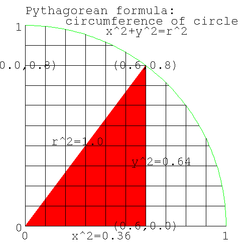 |
Pythagorean formula for circumference of a circle
From Pythagorus' theorem, we know that the distance from the center at (0,0), to any point (x,y) on the circumference of a circle of radius=1, is 1. The square of the distance to the center of the circle (the hypoteneus) is equal to the sum of the squares of the two sides, the lengths of which are given by (x,y). Thus we know that the locus of the circumference of a circle of radius 1 is
x*x + y*y = 1*1 |
| Note | ||||
|---|---|---|---|---|---|
locus: the path traced out by a point moving according to a law. Here's some examples. The circumference of a circle is the locus of a point which moves at constant distance from the center. A straight line is the locus of a point that moves along the path, which is the shortest distance between two points. An ellipse is the locus of a point which moves so that the sum of the distances to two points (the two focii) is constant. (The planets move around the sun in paths which are ellipses. The sun is one of the focii.)
| |||||
In the diagram above if x=0.6, then y=0.8. Let's confirm Pythagorus.
x^2=0.36, y^2=0.64; x^2+y^2=1. |
Rearranging the formula for the (locus of the) circumference, gives y (the height or ordinate) for any x (the abscissa).
x^2 + y^2 = 1^2 y^2 = 1-x^2 y = sqrt(1-x*x) |
i.e. for any x on the circumference, we can calculate y. e.g. x=0.6: what is y?
y = sqrt(1-x*x) = sqrt(1-0.36) = sqrt(0.64) = 0.8 |
If x=0.707, what is y [192] .
The point on the circle with y=0.5: what angle (by eyeball, or by marking off lengths around the circumference) does the line joining this point to the center, make with the x axis [193] .
Similarly we can calculate x knowing y.
x = sqrt(1-y*y) |
The value of π is known to many more decimal places than we can ever use on a 32 bit computer, so there's no need to calculate it again. Instead let's assume that either we don't know its value, or that we want to do the numerical integration on a problem whose answer is known, to check that we understand numerical integration.
The area of a circle is A=pi*r2, giving the area of the quadrant as pi/4. Knowing the locus of the circumference (we have a formula that gives y for any x), we will numerically calculate the area of the circle, thus giving us an estimate of the value of π.
If we divide the x axis into say 10 intervals, we can make these intervals the base of columns, whose tops intersect the highest part of the circle in that slice (which is on the left side of each slice).
Figure 5. Upper Bound of area under slices of a circle
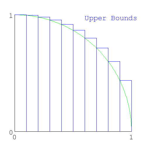 |
Upper Bound of area under slices of a circle
When we add these slices together, we'll get an area that is greater than π; i.e. we will have calculated an upper bound for π.
Here's the set of columns that intersect the lowest part of the circle in each interval (here the lowest part of the circle is on the right side of the slice).
Figure 6. Lower Bounds of area under slices of a circle
 |
Lower Bounds of area under slices of a circle
We can calculate the area of the two sets of columns. If we sum the sets of upper bound columns, we'll get an estimate which is guaranteed to be more than pi/4 and for the set of lower bound colums, a number guaranteed to be less than pi/4.
| Note |
|---|---|
We could have picked the point in the middle of the interval to calculate the area. The answer will be more accurate, but now we don't know how accurate (we don't even know if it's more or less than π). The advantage of the method used here is that we have an upper and lower bound for π, and so we know that the value of π is in this range. We could have used tighter bounds - lower bound by constructing a straight line joining the left and right end of each interval (giving a trapezoid), - upper bound by making a line tangent to the circle. (This is more bother than it's worth, and are left as an exercise for the student.) | |
If we progressively decrease the size of the interval (by changing from 10 intervals, to 100 intervals, to 1000 intervals..) the approximation to a circle by the columns will get better and better giving us progressively better estimates of pi/4. Here's the diagram with 100 slices.
Figure 7. Lower Bounds of area under 100 slices of a circle
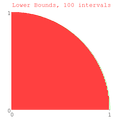 |
Lower Bounds of area under 100 slices of a circle
We have a problem similar to the fencepost error problem: how many heights do we need to calculate if we want to calculate both the upper and lower bounds for 10 intervals. [194] ?
Here's code to generate the heights of the required number of columns (you'll need sqrt(), from the math module). I ran this code in immediate mode, but you can write a file called slice_heights.py if you like.
>>> from math import sqrt >>> for x in range(0,11): ... print x, sqrt(1-1.0*x*x/100) ... 0 1.0 1 0.994987437107 2 0.979795897113 3 0.953939201417 4 0.916515138991 5 0.866025403784 6 0.8 7 0.714142842854 8 0.6 9 0.435889894354 10 0.0 |
Why did I use 11 as the 2nd argument to range() [195] ? What is the "1.0" doing in "1.0*x*x" [196] ?
| Note |
|---|---|
| End Lesson 24 | |
| Note | ||
|---|---|---|---|
Python is a scripting language, rather than a general purpose language. Python can only use integers for loop variables. To feed real values to a loop, python requires a construct like
where x,num_intervals make the real real_number. It's not immediately obvious that the calculations are ranging over values 0.0..1.0 (or more likely start..end). In most languages, real numbers can be used as loop variables, and can use the construct
Here it's clear that x is a real in the range start..end. | |||
Write code pi_lower.py to calculate the lower bound for π using 10 intervals. Use variable names num_intervals, height, area for the number of intervals, height of each column, and for the cumulative area. Start with a loop just calculating the height of each slice, printing the loop index and the height each time. For the print statement use something like
I've been using the single letter variable 'x' as the loop parameter thus far, since it's the loop parameter conveying the position on the x-axis. However loop parameters (in python) are integers, while the x position is a real (from 0.0..1.0). Usually loop parameters (which are integers) are just counters and are given simple variable names 'i,j,k,l...', which are easy to spot in code as they are so short. In this case the loop parameter is the number of the interval (which goes from 0..num_intervals). I tried writing the code with the name "interval" mixed in with "num_intervals" and it was hard to read. Instead I will use 'i'.
print "%d, %3.5f" %(x, height) |
When that's working, calculate the area of each slice and add it to the variable area. The area of each rectangle is height*base. You've just calculated height; what is the width of the base in terms of variables already in the code [197] ?
At the end, print out the lower bound for π with a line like
print "lower bound of pi %3.5f" %(area*4) |
Here's my code for pi_lower.py [198] and here's my output.
0, 0.99499, 0.09950 1, 0.97980, 0.19748 2, 0.95394, 0.29287 3, 0.91652, 0.38452 4, 0.86603, 0.47113 5, 0.80000, 0.55113 6, 0.71414, 0.62254 7, 0.60000, 0.68254 8, 0.43589, 0.72613 9, 0.00000, 0.72613 lower bound of pi 2.90452 |
Do the same for the upper bound of π writing a file pi_upper.py and using variables num_intervals, Height, Area (note variable names for the upper bounds start with uppercase, to differentiate them from the lower bounds variables). Here's my code [199] and here's my output.
0, 1.00000, 0.10000 1, 0.99499, 0.19950 2, 0.97980, 0.29748 3, 0.95394, 0.39287 4, 0.91652, 0.48452 5, 0.86603, 0.57113 6, 0.80000, 0.65113 7, 0.71414, 0.72254 8, 0.60000, 0.78254 9, 0.43589, 0.82613 upper bound for pi 3.30452 |
The two bounds (upper and lower, from the output of the two programs) show 2.9<pi<3.3 which agrees with the known value of π.
The two pieces of code look quite similar. Also note some of the numbers in the outputs are the same (how many are the same [200] ?) We should check for code duplication (in case we only need one piece of code).
Figure 8. Upper and Lower Bounds of area under a circle
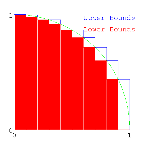 |
Upper and Lower Bounds of area under a circle
Looking at the diagram above which shows upper and lower bounds together, we see the following
- The height of the lower bound in one slice is the same as the upper bound for the next slice to the right.
- The difference between the upper and lower bounds (the series of white rectangles with the arc of the circumference going from the bottom right corner to the upper left corner), when added together, is the same as the height of the left most slice.
Redrawing the diagram, shifting the lower bounds slices one interval to the right shows
Figure 9. Upper and shifted Lower Bounds of area under a circle
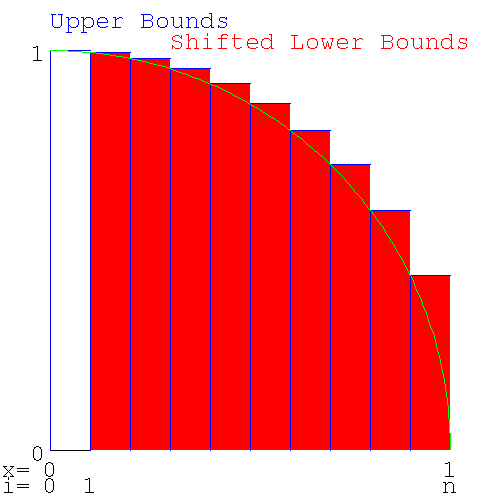 |
Upper and shifted Lower Bounds of area under a circle
This shows that the upper and lower bounds only differ by the area of the left most slice. This means only one loop of code is needed to calculate both bounds. Look in the output of pi_lower.py and pi_upper.py for the 9 numbers in common.
The duplication arises because the lower bound for one interval is the upper bound for the next interval and we only need to calculate it once. The first interval for the upper bound and the last interval for the lower bound are unique to each bound and will have to be calculated separately.
| Note |
|---|---|
| This is a general phenomenon: When calculating a value by determining an upper and lower bound, if the curve is monotonic, you should expect to find values that are used for both the upper and lower bound. | |
Write code (call the file pi_2.py - there is no pi.py anymore) to calculate the area common to both bounds (i.e. except for the two end pieces) in one loop. Use x for the loop control variable (the slice number), h for the height of each slice and a to accumulate the common area. In the loop output the variables for each iteration with a line like
print "%10d %10.20f %10.20f" %(x, h, a) |
After exiting the loop, add the two end areas, one for the lower bound and one for the upper bound to give area and Area and output your estimates of the lower and upper bounds for π with a line like
print "pi upper bound %10.20f, lower bound %10.20f" %(Area*4, area*4) |
Here's the code [201] and here's the output
pip:# ./pi_2.py 1 0.99498743710661996520 0.09949874371066200207 2 0.97979589711327119694 0.19747833342198911621 3 0.95393920141694565906 0.29287225356368368212 4 0.91651513899116798800 0.38452376746280048092 5 0.86602540378443859659 0.47112630784124431838 6 0.80000000000000004441 0.55112630784124427841 7 0.71414284285428497601 0.62254059212667278711 8 0.59999999999999997780 0.68254059212667272938 9 0.43588989435406727546 0.72612958156207940696 pi upper bound 3.304518, lower bound 2.904518 |
giving the same result: 2.9 < pi < 3.3
To get a more accurate result, we now increase the number of intervals, thus making the slices smaller and reducing the jaggyness of the approximation to the circle.
| Note |
|---|---|
| End Lesson 25 | |
| Note | ||||
|---|---|---|---|---|---|
Engineers take pride in being able to do what is called a back of the envelope calculation. While it may take weeks of computer time to get an accurate answer, an engineer should be able to get an approximate answer using only the back of an envelope to do the calculation (extra points are added if you can do it in the elevator between floors). As part of the calculation, you also need to be able determine the accuracy of your answer (is it correct within a factor of 100,10,2, 10%?) or state whether it's an upper or lower bound. If the answer is within reasonable bounds, then it's worth spending a few months and a lot of money to find the real answer. e.g. how long does it take to get from Earth to Mars using the minimum amount of fuel. It's going to be somewhere between the half the time of Earth's orbit and half the time of Mar's orbit (both planets orbit using no fuel at all), i.e. between 6 months and a year - let's make it 9 months. The answer is 8.6 months (Earth-Mars Hohmann trajectory http://www.newmars.com/wiki/index.php/Hohmann_trajectory).
| |||||
Before we change the number of intervals to some large number (like 109), we need some idea of the time this will take. We could change intervals to 10,100... and measure the time for the runs (the quite valid experimental approach) and extrapolate to 109 intervals. Another approach is to do a back of the envelope calculation of the amount of time we'll need. We don't need it to be accurate - we just need to know whether the run will take a second, an hour or a year, to see if it's feasible to run the code with intervals=109. Lets say we use 1G intervals. The calculation goes like this
- our computer has a clock rate of 1GHz, meaning that it can do 1G operations/sec (approximately).
- the for loop is executed once for each interval. Let's say there are 100 operations/loop (rough guess, we could be out by a factor of 10, but that's close enough for the moment)
A 1GHz computer then will take about 100 secs for num_intervals=109. If you have a 128MHz computer, expect the run to be 8 times longer (800secs=13mins). In this case, you may not be able to do a run with num_intervals=109 in class time, but you should be able to do a run with num_intervals=108.
Do multiple runs of pi_2.py increasing num_intervals by a factor of 10-100 each time, noticing the changes in the upper and lower bounds for π. (Comment out the print() statement inside the loop or it will take forever.)
| Note |
|---|---|
| This is a problem with how I wrote the python code. It has nothing to do with numerical integration, but you're going to run into problems like this and you need to know how to get out of them. So we're going to take a little detour to figure this one out. | |
For a large enough value of num_intervals (try 108 or 109, depending on your computer), the program exits immediately with a MemoryError: the machine doesn't have enough memory to run the program. When you have a problem with code, that you've thought about for a while and can't solve, you don't just dump the whole program (with thousands of lines of code) in someone's lap and ask them what's wrong. Instead you pare down the code to the simplest piece of code that will demonstrate the problem and then ask them to look it over. Here's a simplified version of the problem showing the immediate exit:
>>> num_intervals=100000000 >>> height=0 >>> for interval in range(0,num_intervals): ... height+=interval ... Traceback (most recent call last): File "<stdin>", line 1, in ? MemoryError |
| Note | |
|---|---|---|
If I'd gone one step further to
| ||
With a smaller value for num_intervals (try a factor of 10 smaller), this code will now run, but take up much of the machine's memory (to see memory usage, run the program top). I thought that the code was only creating a handful of variables (x, height, num_intervals). In fact range() creates a list (which I should have known) with num_intervals number of values of x, using up all your memory. In all other languages, the code equivalent to
for i in range(0,num_intervals): |
calculates one new number each iteration, and not a list at the start, so you don't have this problem. You don't need a list, you only need to create one value of x for each iteration.
While I was waiting for an answer on the python mailing list, I changed the for loop to a while loop. Here's the equivalent while loop
>>> num_intervals=100000000 >>> height=0 >>> interval=0 >>> while (interval<num_intervals): ... height+=interval ... interval+=1 ... |
which works fine for large numbers of iterations (there doesn't need to be anything in particular inside the loop to demonstrate that a while loop can handle a large number of iterations).
Back to range(): Not only do you run into problems if you create a list longer than your memory can hold, but even if you have infinite memory, there is another upper limit to range(): you can only create a list of length=231
>>> interval=range(0,10000000000) #list 10^10 Traceback (most recent call last): File "<stdin>", line 1, in ? OverflowError: range() result has too many items >>> interval=range(0,10000000000,4) #list of every 4th number of 10^10 numbers = 2.5*10^9 Traceback (most recent call last): File "<stdin>", line 1, in ? OverflowError: range() result has too many items >>> >>> interval=range(0,10000000000,5) #list of every 5th number of 10^10 numbers = 2*10^9 Traceback (most recent call last): File "<stdin>", line 1, in ? MemoryError |
Why did the error change from OverflowError with a list of length 2.5*109 to MemoryError with a list of length 2.0*109?
OverflowError indicates that the size of the primitive datatype has been exceeded. MemoryError indicates that the machine doesn't have enough memory to do that operation (i.e. your machine has less than 2G memory) - python will allow a list of this length, but your machine doesn't have enough memory to allocate a list of this size.
What primitive data type is being used to hold the length of lists in python [202] ?
If the transition from MemoryError to OverflowError had happened between 4.0*109 and 4.5*109, what primitive datatype would python have been using [203] ?
It turns out on a 64 bit system you can still only create a list of length 231.
The python way of overcoming the memory problem of range() is to use xrange() which produces only one value of the range at a time (xrange() produces objects, one at a time, while range() produces a list). Change your pi_2.py to use xrange() and rerun it with a large value of num_intervals. Here's my fixed version of pi_2.py called pi_3.py. The only change to the code is changing range() to xrange() [204] .
| Note |
|---|---|
| Use xrange() whenever you are creating a list of size comparable to the memory in your machine. | |
When coding your goals (in order) are
- get the code to run
- get the code to run correctly
- get the code to run fast
The current code runs correctly, but it runs slowly. Your first attempt at coding up a problem is always like this: you (and everyone else involved) wants to see if the problem can be handled at all. The process of changing code so that it still runs correctly, but now runs quickly, is called "optimising the code".
If you have a piece of software running on a $1M cluster of computers and you can speed it up by 10%, you just saved your business $100k. The business can afford to pay a programmer $100k for a year's work to speed up the program by only 10%. Optimising code is tedious and difficult and you can't always tell ahead of time how successful you'll be. People who optimise code can get paid a lot of money. On the other hand, the people with the money can't tell whether the code needs to be optimised (they think if it works at all, then it's finished) and can't tell a person who can optimise, from one who can't.
If you're selling the software to someone else, then the cost of the extra hardware, needed to run the unoptimised software, is borne by the purchaser and not you, so software companies (unless they have competition) have no incentive to optimise their code. Software companies, just like many businesses, will externalise their costs whenever they can (see Externality http://en.wikipedia.org/wiki/Externality, and Cost_externalizing http://en.wikipedia.org/wiki/Cost_externalizing). With little competition in the software world, there's a lot of unoptimised and badly written code in circulation.
The place to look for optimising, is the lines of code where most of the execution time is spent. If you double the speed of the code where only 1% of the execution time occurs, the code will now take 99.5% of the time, and no-one will notice the difference. It's better to tackle the part of the code where 99% of the time is spent. Doubling the speed there will halve the run time. Places in the code where a lot of time is spent are loops that are run many times (or millions of times). In pi_3.py the program is only a loop and it's running 109 times.
Let's look at the loop in pi_3.py.
Pre-calculate constants:
How many times in the loop is num_intervals*num_intervals calculated? How many times do you need to do it [205] ?
We won't modify pi_3.py till we've figured out the optimisations we need. Instead we'll use this simple code (call it test_optimisation.py) to demonstrate (and time) optimisation. Remember that the timing code measures elapsed (wall clock) time rather than cpu time (i.e. if your machine is busy doing something else, the time won't be valid). If your computer is about 200MHz, run the program with num_intervals=105; if you have a 1GHz machine, use num_intervals=106.
#! /usr/bin/python #test_optimisation.py from time import time num_intervals=100000 sum = 0 print " iterations sum iterations/sec" start = time() for i in xrange(0,num_intervals): sum+=(1.0*i*i)/(num_intervals*num_intervals) finish=time() print "unoptimised code: %10d %10.10f %10.5f" %(num_intervals, sum, num_intervals/(finish-start))Why do I print out the results num_intervals, sum at the end when I only need to print out the speed? It's to show that the code, whose speed I'm measuring, is doing what it's supposed to be doing. What if my loop was coded incorrectly and was doing integer, rather than real, division? As a check, I should at least get the expected value for sum in all runs.
Add another copy of the loop below the unoptimised loop (including the timing and print commands), recoded so that num_intervals*num_intervals is only calculated once.
Note When you modify code, comment out the old code, rather than deleting it. Later when you're done and the code is working properly, you can delete the code you don't want. Right now you don't know which code you're going to keep. Here's my new version of the loop (with the original code commented out in the revised version of the loop). This is a stand-alone piece of code. You will just be adding the loop part to test_optimisation.py. [206] .
Initially I handled the different versions of the loop by re-editing the loop code, but it quickly became cumbersome and error prone. Instead, I spliced the different versions of loop code into one file and ran all versions of the loop together in one file. Here's what my code looked like at this stage [207] .
Note from Joe: you can skip this part (it shows that division by reals which are powers of 2, doesn't use right shifting). Long division is slow - pt1 (can we right shift instead?).
We've been using powers of 10 for the value of num_intervals. We don't particularly need a power of ten, any large enough number would do. Dividing by powers of 10 requires long division, a slow process. Integer division by powers of 2 uses a right shift, a much faster process. If real division is like integer division, then if we made num_intervals a power of 2, the computer could just right shift the number. In your test_optimisations.py make a 3rd copy of your loop, using the new value of num_intervals
If your computer is about 200MHz, run the program with num_intervals=105 and num_intervals=217 (both have a value of about 100,000). If you have a 1GHz machine, use num_intervals=106 and 220.
There's no change in speed, whether you're dividing by powers of 2 or powers of 10. While integer division by powers of 2 uses right shifting, division by reals uses long division, no matter what the divisor (the chances of a real being a power of 2 is small enough that python - and most languages - just has one set of code for division).
Long division is slow - pt2 (but multiplication is fast).
Why is multiplication fast, but division slow? Division on computers uses long division, the method used to do division by hand. If you divide a 32 bit number by a 32 bit number, you'll need 32 steps (approximately), all of which must be done in order (serially). Multiplication of the same numbers (after appropriate shifting) is 32 independant additions, all of which can be done at the same time (in parallel). If you're going to use the same divisor several times, you should instead multiply by the reciprocal.
Rather than dividing by num_intervals_squared once for each iteration, we should multiply by the reciprocal. Make another copy of your loop, this time multiplying by the reciprocal of num_intervals_squared. Here's my stand-alone version of the code (add the loop, timing commands and print statements to the end of test_optimisations.py) [208] . Do you see any change in speed?
Here's my test_optimisation.py [209] and here's the output run on a 200MHz machine
pip:# ./test_optimisation.py iterations sum iterations/sec unoptimised code: 1000000 0.0000010000 38134.77894 precalculate num_intervals^2: 1000000 0.0000010000 63311.38723 multiple by reciprocal: 1000000 0.0000010000 88156.25065 |
showing a 2.5-fold increase in speed.
| Note |
|---|---|
| End Lesson 26 | |
Don't alter your pi_3.py; you aren't finished with test_optimisations.py yet.
Computers have a large but limited range of numbers they can manipulate. We're calculating π, whose value lies well in the range of numbers that computers can represent. However numerical methods, like we are using here, use values that are very small (and the squares of these numbers are even smaller). Other codes can divide small numbers by large numbers, large numbers by small numbers, square numbers that are smaller than the square root of the smallest representable numbers, or square numbers that the are bigger than the square root of the biggest representable numbers. You'll wind up with 0 instead of a small number or NaN (not a number, the computer result of dividing by 0). If you're close to the edge there, you drop significant figures and wind up with an inaccurate answer. Your rocket may not blow up for 10 launches, then one day when the breeze is coming from a different direction, the guidance system won't be able to correct and your rocket will blow up.
With the range of numbers we're using in the numerical integration, we're not going to have this problem. However you're writing code that for a different range of numbers will have this problem. Someone could swipe your code and use it for a new range of inputs, or you could re-use it in another piece of code. You want to write the code to minimise problems in the distant future. Here's where this problem shows up in our code
(1.0*x*x)/(num_intervals*num_intervals) |
Depending on x, this is a small number squared, over a large number squared (x*x might evaluate to 0.0 and the division by num_intervals*num_intervals would be irrelevant; or num_intervals might be large, causing num_intervals*num_intervals to overflow i.e. NaN) - a disaster with your rocket's name on it. Instead you should write
(1.0*x/num_intervals)^2 |
Numbers and their scaling constants should not be separated. In computing, dividing a data value by some appropriate scaling constant is called normalisation. The word "normalisation" is used in different places to mean different things (unfortunately). Where else have we seen the term [210] ? You can take "normalised" to mean "anything that fixes up numbers so that something awful doesn't happen". What that may mean in any particular situation, you'll have to know.
The term used in science/engineering is "reduced" (rather than "normalised"), where the reduced value is dimensionless. Say a machine/system can do a maximum of 1000 operations/hr. If it's doing 500 operations/hr, its reduced speed is 0.5 (not 0.5 of its maximum speed, just 0.5 i.e. a number). Rather than refer to the speed of a plane (which has the dimensions of l/t), you can refer to its Mach number (the speed of the plane/speed of sound, this is dimensionless). The speed of sound depends on temperature. The temperature of air varies with altitude, so the speed of sound varies with altitude. Aerodynamics, especially near the speed of sound depends on the Mach number and not the speed (you'll need your speed to know when you'll arrive at your destination). If you're studying the aerodynamics of a plane at different altitudes, you want to know the Mach number.
In computations, often there will be dimensionless terms like x/y (which might be speed/speed of sound). In this case while each of the variables x,y might have a large range of values (e.g. 10**-160 to 10**160), the range of x/y might be from 10**-1 to 10**1.
Let's say we have a calculation which requires the value of (x/y)2 when each of x,y have large ranges, but x/y has a small range. Here's how the ant climbing a hill, (floating point precision) looking for the highest point, gets stuck and starts wandering around aimlessly.
#small numbers (you have to guard against this possibility when doing optimisation problems) >>> x=10**-161 >>> x*x 9.8813129168249309e-323 >>> x=10**-162 >>> x*x #underflow: x*x is too small to be represented by a 64-bit real 0.0 >>> interval=10**-150 >>> (x*x)/(num_interval*num_interval) #underflow: invalid answer 0.0 >>> (x/num_interval)*(x/num_interval) #normalised number gives valid answer 9.9999999999999992e-25 #the correct answer is 10^-24, this answer is near enough #big numbers (this doesn't happen a real lot) >>> num_interval=1.01*10**154 >>> num_interval*num_interval 1.0201e+308 >>> num_interval=1.01*10**155 #if I don't have the 1.01, the number will be an integer >>> #python can have abitrarily large integers >>> #and you'll get the correct answer >>> num_interval*num_interval #squaring a large number inf #overflow >>> x=1.01*10**150 #squaring a slightly smaller number >>> x*x 1.0201000000000001e+300 >>> (x*x)/(num_interval*num_interval) #unnormalised division 0.0 #wrong answer >>> (x/num_interval)*(x/num_interval) #normalised division 1.0000000000000002e-10 #correct answer |
Whenever you have
y=(a*b*c)/(e*f*g) |
figure out which denominator terms normalise which numerator term (you'll know from an understanding of the physics of the problem). You'll wind up changing the code to something like this
y=(a/e)*(b/f)*(c/g) |
With the numbers we're using in the numerical integration, we aren't getting any benefit from using reduced numbers. None of the numbers under or overflow on squaring. However reduced numbers should always be used, just as seat belts should be used in cars. Here's the range of numbers involved
- loop counter: i: 1..num_intervals (1-109)
- 1.0/num_intevals2: 10-18
- reduced variable i/num_intevals: 1.0/num_intervals.. 1.0 (10-9..1.0)
- square of reduced variable (i/num_intevals)2: (1.0/num_intervals)2.. 1.02 (10-18..1.0)
We're dealing with numbers 10-18..1.0 whether we reduce or not.
Here's a case when reduced variables helps.
- range of x: 10-160..10160
- range of y: 10-140..10140
- range of x/y: 10-20..1020
Here if we square x,y separately, we'll get an under or overflow. If we use reduced numbers, we'll get a correct answer.
Why did I get you to use reduced numbers when you don't need them? It's a good programming practice. You never know what someone else is going to do with your code. When another coder reads your code, he can tell that you know what you're doing and he won't have to have to look for stupid coding errors. This sort of code gives you good programming cred to people reading your code. You need to fix problems before they happen (not after). This country has blown up two Space Shuttles because people didn't fix problems when they came up to be fixed. You don't want to write code that blows up Space Shuttles.
In computers, division is done by long division, the same way you divide by hand. Long division is slow compared to multiplication, which on a computer (with special hardware) can be done in two steps. In a loop, if you divide by a constant, it's faster to multiply by the reciprocal.
#loop, slow way a=h/num_intervals #faster way interval=1.0/num_intervals #outside loop #loop a=h*interval |
Add another section with a loop to test_optimisations.py using the reduced number x/num_intervals (since 1/num_intervals is used several times, you should multiply by the reciprocal, and so the code will actually use x*interval). Here's the code [211] and here's the ouput.
./test_optimisation.py iterations sum iterations/sec unoptimised code: 1000000 0.0000010000 37829.84246 precalculate num_intervals^2: 1000000 0.0000010000 63759.14714 multiply by reciprocal: 1000000 0.0000010000 99322.31288 normalised reciprocal: 1000000 0.0000010000 60113.31327 |
Here's my final version of test_optimisations.py [212] .
Because you're reducing numbers, you can no longer take advantage of the precalculated square, and your code is slower. In general, you don't care if normalisation slows down the code; you'd rather your rocket's navigation system worked correctly but slowly, than crashing the rocket quickly. If you're doing the runs yourself, and you know that the data is well conditioned and doesn't have to be reduced, you can do a run that takes a week instead of 10days. However, in 6 month's time, if your rocket blows up with someone's $1B satellite on board, no-one's going to be impressed when they find that your code didn't normalise. If your code will be released to a trusting and unsuspecting world, to people who will feed it any data they want, you must normalise.
The optimisations we tested were
- constants in a loop need to be precalculated
- multiply by constants, not divide
- normalise (reduce) variables
If the loop had been longer (say 50 lines long), with lots of other calculations, then moving the generation of the constant out of the loop may not have made much difference. However the optimisations shown here should be done as a matter of course; they will assure anyone reading your code, that you know what you're doing.
The optimisations shown here are relatively routine and are regarded as normal programming practice, at least for a piece of code that takes a significant fraction of the runtime (e.g. a loop which is run many times). You wouldn't bother optimising if the lines of code were only run a few times. The unoptimised code that I've presented to you was deliberately written to be poor code so that you could make it better.
| Note |
|---|---|
End Lesson 27: At this stage I'd left the students with the results of running test_optimisation.py, expecting them to figure out on their own, the optimisations that would be incorporated into the numerical integration. By the next class, they couldn't even remember the purpose of reducing numbers, so I went over this lesson again, and had them disect out the optimisation that would be transferred to the numerical integration. | |
Which optimisations are you going to use in the numerical integration? We have tried these loops:
sum = 0
#unoptimised
for i in xrange(0,num_intervals):
sum+=1.0/(num_intervals*num_intervals)
#faster
#precalculate constants (here num_intervals^2)
num_intervals_squared=num_intervals*num_intervals
for i in xrange(0,num_intervals):
sum+=1.0/num_intervals_squared
#fastest
#multiply by constants, don't divide
interval_squared=1.0/num_intervals_squared
for i in xrange(0,num_intervals):
sum+=1.0*interval_squared
#safe, about the speed of "faster", not "fastest"
#use reduced numbers
interval=1.0/num_intervals
for i in xrange(0,num_intervals):
sum+=(1.0*interval)**2
|
The optimisations we can use for the final code are
- reduced numbers: We have to use these for safety.
- Once you choose reduced numbers, you can no longer precalculate num_intervals2 (or its reciprocal) because num_intervals is subsumed into the reduced number.
- You can still precalculate the reciprocal of num_intervals to make your reduced number.
We must use reduced numbers for safety. Once we've made this choice, the only other optimisation left is to multiply by the inverse of num_intervals. We can't use any of the other optimisations. We don't get the best speed, but we will get the correct answer for a greater range of x, num_intervals
As a programmer, if you're selling your code, you are in somewhat of a bind here. If your code is compared to a competitor's, which uses all the speed optimisations, and which doesn't reduce their numbers, your code will run at half the speed of the competition. It would take quite a sophisticated customer (one who can read the code) to understand why your code is better. In my experience, people who want the program, rarely know the back from the front of a computer, much less understand the trade-offs involved in coding for safety or speed. If you tell the customer that you can make your code run fast too, but it just won't be safe, and they buy your code and it does blow up a rocket or kill a patient in a hospital, they'll still take you to court for shoddy programming. The "poor unknowing customer", who bought the code knowing full well that wasn't safe, won't be blamed.
Solaris (the unix variant used as the OS on Sun's computers) is slow compared to their competitor's OSs and it's disparaged by calling it "Slolaris". It throws up a lot of errors in the logs (say when there's a network problem), while the logs of a competitor's machine, on the same network, seeing the same problems, are empty. People in the know defend Solaris saying it is slow because it's safer and that the other OSs are seeing errors too, but aren't reporting them. The people on the other machines say "my machine isn't having any problems, Slolaris is having the problem!". Expect this if you write good code.
Here's the way out of the bind.
- You have sophisticated users: This likely scenario for this would be if you wrote some code and put it out on the internet, under a GPL License, saying "here's code which does X, and here's the tests I put it through. Have fun." Your users will expect you know what you're doing and will go find things to do with it and using it out of any bounds that you ever thought about. You'll use safe programming.
-
You have a paying customer who doesn't know anything about programming or computers.
They want code that runs fast,
because they're using the cheapest possible hardware to save costs.
(Everyone wants to save costs, you only have to give token acknowledgement of this.
Some people want to save costs in a way that makes it expensive in the long run.)
You say
I can make it run fast or I can make it run safe. Here is the range of parameters under which I've tested it. If you stay in this range you can run the fast code. If you go outside this range you'll need the safe code.
Now no matter which one they want, you have them write it into the specifications (including the caveats as to what might happen if they used the code outside the test conditions), so that legally you can say that you wrote what they wanted and they paid for what they asked for.
We now need to incorporate the optimisations, and time our π calculation runs. Code takes a while to load from disk. If it's just been run, a subsequent run will load faster (the disk cache knows where the file is or will still have the file cached in memory). Speed then will be affected by how long since the code was last run (after about 15 secs, the cache has been flushed). When you do several runs, you may notice that the first run is slow.
Copy pi_3.py to pi_4.py and include the optimisations that we found to be useful for this code (hint [213] ). Here's my version of pi_4.py [214] .
Table 4. Results of optimising calculation of π by numerical integration
| code optimisation | speed, iterations/sec (computer 1) | speed, iterations/sec (computer 2) |
|---|---|---|
| none (base case) | 16k | 73k |
| all | 24k | 105k |
| Note |
|---|---|
| This section hasn't been presented in class. It was written while the kids are writing their presentations. | |
Once we have the upper and lower bounds, the value of π comes by comparing the two numbers and accepting from the left, the numbers that match. As soon as we find a non-match, we discard the remaining digits. Since we're calculating π only once, we could match by hand and write down the answer. However your high school wants you to know array operations, so we'll use array operations to do the matching. In python, arrays are implemented with lists. If you need to, first refresh your memory of list operations lists and list of lists. Then go to arrays. Here you'll learn about arrays (you don't need to know all the material in this section to do the following section here, but your school wants you to understand arrays, and it's a good opportunity to get aquainted with them). Then go to the following section turning reals into strings and return here.
Lets do the match by finding the char elements of a string. (I wish to thank members of the North Carolina Zope/Python User Group for help here. There is a neater solution using the python specific zip() which I don't want to use - I'm only using code that will work in any language.) Write code compare_reals.py that does the following
-
initialises
- two reals (call them real_lower, real_upper) giving them a pair of values from lower and upper bounds
- a string pi_result to hold the matching digits of the two reals
- put the string representations of the two reals into string_lower,string_upper
- What happens if you compare strings of different lengths [215] ? To handle the case when the two strings are of different length, find the length of the shorter string (use the python function len(), which returns an integer, to find the length of a string). Assign the length of the shortest string to the variable shorter.
- iterates (loops) over the two strings comparing the char elements at that position in the string.
- when the two chars match, add that char to pi_result
-
when the loop finds the first non-matching pair,
execute the python command break which exits the loop,
thus preventing the loop from adding matching chars further down the string.
The code with the break statement will look like this
for i in range(start, finish): if (char i from string_1==char i from string_2): add char to output string else: break # exit the for loop
- leave pi_result as a string and output it to the screen.
Should you output a string or a real? With the upper and lower bounds being reals, you might expect to write code returning π as a real. However if the string was "3.141", after conversion to a real it might be 3.140999999999995. With correct formatting in the print statement, it might be possible to output this as 3.141, but you would have to know ahead of time the number of places to output. It's pointless to do this when you already have the correct number of places in the string form of π.
| Note |
|---|---|
|
Optional: If you wanted to output a real for pi_result.
If you were to output (or return) a real, you'd use the function float() on the string. Test your code when no digits match (what is float("")?). Will your rocket crash and burn [216] ? | |
Here's my code [217] . What is the order of the algorithm? i.e. if the length of the strings are increased by a factor of n, will the runtime increase by n times or n2 times (or some other function of n) [218] ?
The value of π is truncated to the number of digits presented. It would be more accurate if we rounded the number up or down. Can we do that? If the first non-matching digits are both 5 or above, we can definitely round up. If the first non-matching digits are both 4 or below, we can definitely round down. What if one digit us 4 and the other 7? We can't say anything. We can't have a scheme where the last digit may be rounded or may be truncated, but we can only tell by looking up the original computer print out. Our only choice is to say that the value of π is truncated to the quoted number of places.
Copy the code to compare_reals_2.py. Make the code into a function string longest_common_subreal(real,real) (i.e. takes parameters of two reals, and returns a string). Change the names of variables to be more generic i.e. string_lower becomes string_1, so that the code will apply to any situation, not just to upper and lower bounds. In main() call the function with two reals (use typical values for upper and lower bounds) and print out the result. Here's my code [219] .
Copy pi_4.py to pi_5.py. Add longest_common_subreal() to the code, so that it outputs the truncated string for the estimate for π. Here's my code [220] .
Using pi_5.py pick a high enough value for num_iterations to get meaningful output (it looks like I used num_iterations=109, you won't have time to run this in class). Do runs starting at num_intervals=1 (for Cygwin under Windows, the timer is coarse and will give 0 for num_intervals<10000), noting the upper and lower bounds for π. We want to see how fast the algorithm converges and get progressively tighter bounds for π. Here's my results as a function of num_intervals.
| Note |
|---|---|
| End Lesson 28 | |
Table 5. π (and upper and lower bounds) as a function of the number of intervals
| intervals | lower bound | pi (truncated) | upper bound | program time,secs | loop time,secs |
|---|---|---|---|---|---|
| 100 | 0.0 | 4.0 | 0.030 | 0.000022 | |
| 101 | 2.9 | 3.3 | 0.030 | 0.000162 | |
| 102 | 3.12 | 3.1 | 3.16 | 0.030 | 0.000995 |
| 103 | 3.139 | 3.1 | 3.143 | 0.040 | 0.0095 |
| 104 | 3.1414 | 3.141 | 3.1417 | 0.13 | 0.094 |
| 105 | 3.14157 | 3.141 | 3.14161 | 0.97 | 0.94 |
| 106 | 3.141590 | 3.14159 | 3.141594 | 9.51 | 9.45 |
| 107 | 3.1415924 | 3.141592 | 3.1415928 | 95.1 | 95.1 |
| 108 | 3.14159263 | 3.1415926 | 3.14159267 | 948 | 947 |
| 109 | 3.141592652 | 3.14159265 | 3.141592655 | 9465 | 9464 |
| 1010 - not an int, too big for xrange() | - | - | - | - | - |
We're doing runs that take multiples of 1000sec. Another useful number: how long is 1000 secs [221] ?
For large enough number of intervals, the running time is proportional to the number of intervals. It seems that the setup time for the program is about 0.03 sec and the setup time for the loop stops proportionality at about 10 intervals.
The difference between the upper and lower bound of π is 1/num_intervals (the area of the left most slice). If we want to decrease the difference by a factor of 10, we have to increase num_intervals (and the number of iterations) by the same factor (10), increasing the running time by a factor of 10. If it takes an hour to calculate π to 9 places, it will take 10hrs to calculate 10 places. With about 10,000 hours in a year, we could push the value of π out to all of 13 places. We'd need 100yrs to get a double precision value (15 decimal places) for π.
Here's the limits we've found on our algorithm:
Table 6. Limits to calculating π by numerical integration
| limited item | value of limit | reason for limit | fix |
|---|---|---|---|
| range() determines max number of intervals | 100M-1G | available memory | use xrange() |
| time | 1hr run gives π to 9 figures | have a life and other programs to write | faster algorithm |
| precision of reals | 1:1015 | IEEE 754 double precision for reals | fix not needed, ran out of time first |
If someone wanted us to calculate π to 100 places, what would we do [222] .
Calculating π to 100 places by numerical integration would require 10100 iterations. Doing 109 calculations/sec, the result would take 10(100-9)=1091 secs. To get an idea of how long this is, the Age of the Universe (http://en.wikipedia.org/wiki/Age_of_the_universe)=13Gyr (another useful number) =13*109*365*24*3660=409*1015 secs. If we wanted π to 100 places by numerical integration, we would need to run through the creation of 10(100-9-17)=1074 universes before getting our answer.
As Beckmann points out, quoting the calculations of Schubert, we don't need π to even this accuracy. The radius of the (observable) universe is 13*109 lightyears = 13*109*300*106 * 365*24*3600=1026m=1036Å. Assuming the radius of a hydrogen atom is 1Å, then knowing π to 102 places, would allow us to calculate the circumference of the (observable) universe to 1026/10100=10-64 times the radius of a hydrogen atom.
Despite the lack of any practical value in knowing π to even 102 places, π is currently known to 1012 places (by Kanada).
We calculated π by numerical integration, to illustrate a general method, which can be used when you don't have a special algorithm to calculate a value. Fortunately there are other algorithms for finding π. If it turned out there weren't any fast algorithms for π some supercomputer would have been assigned to calculate 32-,64- and 128-bit values for π long ago; and they'd now be stored in libraries in our software.
While there are fast algorithms to calculate π, there aren't general methods for calculating the area an arbitary curve, and numerical integration is the method of choice. It's slow, but often it's the only way.
It can get even worse than that: sometimes you have to optimize your surface. You numerically integrate under your surface, then you make a small change in the parameters hoping for a better surface, and then you do your numerical integration again to check for improvement. You may have to do your numerical integration thousands if not millions of times, before finding your optimal surface. This is what supercomputers do: lots of brute force calculations using high order (O(n2 or worse) algorithms, which are programmed by armies of people skilled at optimisation. People think that supercomputers must be doing something really neat, for people to be spending all that money on them. While they are doing calculations for which people are prepared to spend a lot of money, the computing underneath is just brute force. Whether you think this is neat or not is another thing. Supercomputers are cheaper than blowing up billion dollar rockets, or making a million cars with a design fault. Sometimes there's no choice: to predict weather, you need a supercomputer, there's no other way anymore. Unfortunately much of supercomputing has been to design better nuclear weapons.
I said we need a faster algorithm (or computer). What sort of speed up are we looking for? Let's say we want a 64-bit (52-bit mantissa) value for π in 1 sec. If using numerical integration, we'd need to do 252iterations=4*1015=1015.6 iterations. A 1GHz computer can go 109 operations/sec (not iterations/sec, but close enough for the moment; we're out by a factor of 100 or so, but that's close enough for the moment). We'd need a speed up of 1015.6-9.0=6.6. If we instead wanted π to 100 places (and not 15 places) in 1sec, we'd need a further speed up of 1085. There's no likelihood of achieving that sort of speed-up in computer hardware anytime real soon. Below let's see what sort of speed up we can get from better algorithms.
| Note |
|---|---|
| Again for convenience let's assume that there is one real operation/iteration (or per interval) in the loop calculating π (in fact there are about 10). | |
We now have a value for π. As with all answers, we aren't home yet; we first have to know how good our answer is (i.e. we need an estimate of the errors too). Usually finding/calculating the errors in an answer takes longer than calculating the answer.
Due to the limited precision (32,64 bit) of registers used in computer real operations, rounding errors can (will) occur in every real operation and will affect the result. In the worst case, every floating point operation will have a rounding error and the errors will add, giving us 1 error for every operation.
| Note |
|---|---|
| (In real life, not all calculations will result in a rounding error, and many roundings will cancel. But without a detailed analysis to find what's really going on, we have to assume the worst case.) | |
These errors are seen in the rightmost (least significant) bits of the number/mantissa. For every doubling of the number of intervals (which doubles the number of iterations), an extra bit of error is added at the rightmost end of the upper and lower bounds.
Here's a diagram of the lower bounds calculation after 28 iterations on a 32 bit machine (23 bit mantissa). The least significant 8 bits have errors due to rounding.
| Note |
|---|---|
| Joe: FIXME: do you get the same answer if you have 2^8 intervals and do 2^8 iterations, and in the case where you do 2^8 iterations of a 2^32 interval problem? | |
lower bounds: llllllllllllllleeeeeeee
| | |
20 10 0
l - lower bounds value
e - bit in error due to rounding
|
We've found that increasing the number of intervals by a factor of 10, gives us one more place where the upper and lower bounds match i.e. for every doubling of the number of intervals, an extra bit is added to our value for π. Thus as our calculation proceeds, for every doubling of the number of intervals, an extra bit on the left hand end of the register matches in the upper and lower bounds estimates, allowing us to add an extra bit to the value of π. Thus whenever an error bit is added to the right hand end of the register (the least significant end). an extra bit of precision is added on the left of the register (the most significant end) to our value of π.
Here's a diagram showing the bits in the 23 bit mantissa (32 bit machine) for the upper and lower bounds after 28 iterations. Note that 8 bits match on the left end, giving us the value for π to 8 bits, while 8 bits of rounding error have accumulated on the right end.
upper bounds: mmmmmmmmuuuuuuueeeeeeee
lower bounds: mmmmmmmmllllllleeeeeeee
| | |
20 10 0
m - matching (correct value for pi)
l/u - lower/upper bounds value
e - bit in error due to rounding
|
With a sufficient number of intervals, the error bits and the good bits will meet in the middle. When this occurs you've calculated π to the maximum accuracy for that mantissa size. The number of intervals required to do this is the integer that fits into half the mantissa width.
Here's the maximum possible number of places for π that can be calculated by numerical integration, for various machine bit widths.
Table 7. effect of bit width on maximum number of places for π
| bit width | mantissa | correct bits (on left) | error bits (on right) | iterations | time |
|---|---|---|---|---|---|
| 32 | 23 | 11 | 11 | 211≅103 | 9.5msec |
| 64 | 52 | 26 | 26 | 226≅108 | 16mins |
| 128 | 112 | 56 | 56 | 256≅1019 | 1032yr |
The maximum accuracy of π that can be calculated on 32,64 or 128 bit computers by numerical integration, is 11,26,56 bits (≅3,8,19 decimal places), taking 9msec, 16mins and 1032yr respectively.
For the 32 and 64 bit machines, we need to make sure that we don't run the calculations any longer than needed, otherwise correct bits will be overwritten by errors. (For the 128 bit machine, there won't be enough time, to get to the maximum number of bits.) If the number if intervals is increased past this point, then errors coming from the right end of the register, will overwrite the already calculated good values of π sitting at the left end of the register.
Our calculation of π ran for 109 (≅ 230) iterations/multiplication/additions. This table shows the combined effect of the register bit width (size of reals) and the rounding errors on the result.
Table 8. effect of size of reals and rounding errors on the result for 109 ≅ 230 iterations
| rounding error, bits | real size | mantissa size | correct bits | u/l bounds bits | error bits | correct decimal digits |
|---|---|---|---|---|---|---|
| 30 | 32 | 23 | 0 (all 23 bits are garbage) | 0 | 23 (23<30) | - |
| 30 | 64 | 52 | 22 (8 good bits are overwritten) | 0 | 30 | 7 |
| 30 | 128 | 112 | 30 | 52 (112-60) | 30 | 9 |
In the case of the 23 bit mantissa, all 23 bits are overwritten by 30 bits of rounding errors. In the case of the 52 bit mantissa, the 30 error bits overwrite 8 of the good bits of π that were being calculated in the left most bits and we are left with only 22/3=7 correct decimal places. In the 128 bit case, 30 error bits were produced, 30 good bits were produced and the 52 bits in the middle hold values for the upper and lower bounds.
The error is relative to the number, rather than an absolute number. For slice heights which are less than half of the radius of the quadrant, the error in the heights will be reduced to one half. In this case approximately half the errors will not be seen (they will affect digits to the right of the last one recorded). We have two factors which each can reduce the number of rounding errors by a factor of 2 (half of the errors underflow on addition, and half of the additions don't lead to a rounding error). It's possible then that the worst case errors are only 29 bits rather than 30 bits.
Still it's not particularly encouraging to wait for 109 iterations, only to have to do a detailed analysis to determine whether 29 or 30 of the 52 bits of your mantissa that are invalid. If we did decide to calculate π to 15 decimal places (64 bit double precision, taking 100yrs), doing 1015 operations, what sort of error would we have in our answer [223] ? One of the reasons to go to 64 (or 128) bit registers, is to have a large enough representation of the number that there is room to store all the errors that accumulate, while getting enough correct digits to get a useful answer.
In most cases with numerical integration, we don't know the answer (otherwise we wouldn't be doing the calculation). In this case our answer is the known π so we can use the known value to check our result. Our answer agrees with the known value of π to 9 rather than 7 places. This tells us that we didn't have the worst case errors. In fact we had about 100 times less errors than the worst case. Why was this? Was it due to skillful programming on our part? No; it was just dumb luck - most of the errors cancelled. We can expect as many rounding errors to round down as round up, so we should expect most of them not to be seen. However to know the number of errors we did get, we would need a more complicated error analysis than we've done here.
When we present our value for π from the numerical integration, what accuracy do we give; 7 places or 9 places? We found that the upper and lower bounds agreed to 9 places, so you might think that we can give 9 places. However our error analysis shows that in the worst case only 7 of these places are correct. We have to give our answer to 7 places. (Remember if we were determing the value of π by numerical integration, we wouldn't know its real value.)
We've gone through this numerical integration algorithm in great depth. Back when computers were first being used for modelling and numerical integration, all algorithms were new and they were explored in great depth to analyse speed and errors. Nowadays numerical integration is well understood and no-one would go through their algorithm in the detail we have just done here. They just know that if it's brute force and many iterations, then they'll have to run the code on a 128 bit computer. If you're working in that environment, the 128 bit computers will already be there and you will likely not even think about the number of bits you need (or have a choice of the bit width). (Supercomputing has been using 128bit reals since the 1970s.)
This section was originally designed to illustrate numerical integration. Numerical integration isn't practical for π: it's too slow, and has too many errors. We need another (quicker) algorithm, where most of the 52 bits of the mantissa (in a 64 bit machine) are valid. Since we've got numerical integration covered, let's look at other algorithms for calculating π.
The ancient Egyptians in 2500BC had a value for π accurate to 0.04% (see History of π http://en.wikipedia.org/wiki/Pi#History). The first attempts to calculate a value (by Archimedes, 287-212 BC) used numerical integration. Archimedes drew two sets of polygons, inscribing and circumscribing a circle (to get a lower and upper bounds) (see Archimedes' Polygons http://en.wikipedia.org/wiki/Pi#Geometrical_period) and by increasing the number of sides of the polygon, was able to get a value of π accurate to 4 places. It wasn't till the invention of calculus almost 2000yrs later, that faster algorithms were found to calculate π
There are many mathematical identities involving π and many of them are fast enough to be useful for calculating π. Here's one discovered independantly by many people, but usually attributed to Leibnitz and Gregory. It helped start of the rush of the digit hunters (people who calculate some interesting constant to large numbers of places).
pi/4 = 1 - 1/3 + 1/5 - 1/7 + 1/9 - ... |
Swipe this code with your mouse, calling it leibnitz_gregory.py.
#! /usr/bin/python # #leibnitz_gregory.py #calculates pi using the Leibnitz-Gregory series #pi/4 = 1 - 1/3 + 1/5 - 1/7 + 1/9 - ... # #Coded up from #An Imaginery Tale, The Story of sqrt(-1), Paul J. Nahin 1998, p173, Princeton University Press, ISBN 0-691-02795-1. large_number=10000000 pi_over_4=0.0 for x in range(1, large_number): pi_over_4 += 1.0*((x%2)*2-1)/(2*x-1) if (x%100000 == 0): print "x %d pi %2.10f" %(x, pi_over_4*4) # leibnitz_gregory.py------------------------- |
In the line which updates pi_over_4, what are the numerator and denominator doing [224] ? Run this code to see how long it takes for each successive digit to stop changing. How many iterations do you need to get 6 places (3.14159) using Leibnitz-Gregory and by numerical integration [225] ?
Newton (http://en.wikipedia.org/wiki/Isaac_Newton), along with many rich people, escaped London during the plague (otherwise known as the Black Death http://en.wikipedia.org/wiki/Black_Death, which killed 30-50% of Europe and resulted in the oppression of minorities thought to be responsible for the disease) and worked for 2 years on calculus, at his family home at Woolsthorpe. There he derived a series for π which he used to calculate π to 16 decimal places. Newton later wrote "I am ashamed to tell you to how many figures I carried these computations, having no other business at the time". We'll skip Newton's algorithm for π as it isn't terribly fast.
Probably the most famous series to calculate π is by Machin - see Computing Pi (http://en.wikipedia.org/wiki/Computing_%CF%80), also see Machin's formula (http://milan.milanovic.org/math/english/pi/machin.html).
pi/4 = 4tan^-1(1/5)-tan^-1(1/239) |
Machin's formula gives (approximately) 1 significant figure (a factor of 10) for each iteration and allowed Machin, in 1706, to calculate π by hand to 100 places (how many iterations did he need?). The derivation of Machin's formula requires an understanding of calculus, which we won't be going into here. For computation, Machin's formula can be expressed as the Spellbach/Machin series
pi/4 = 4[1/5 - 1/(3*5^3) + 1/(5*5^5) - 1/(7*5^7) + ...] - [1/239 - 1/(3*239^3) + 1/(5*239^5) - 1/(7*239^7) + ...] |
250 years after Machin, one of the first electronic computers, ENIAC, used this series to calculate π to 2000 places.
| Note |
|---|---|
| End Lesson 29 | |
This series has some similarities to Gregory-Leibnitz. There are two grouping of terms (each within [...]). In the first grouping note the following (which you will need to know before you can code it up)
- There is an alternating sign
- There is are terms 1/1, 1/3, 1/5..., which you also had in Leibnitz-Gregory.
- There is are terms (1/5)1, (1/5)^3, (1/5)5... How would you produce these in a loop?
In each term in the series consider
- which number(s) are variable and will have to come from the loop variable
- which number(s) are constants
The second set of terms is similar to the first with "239" replacing "5". The second set of terms converge faster than the first set of terms (involving "5"), so you don't need to calculate as many of the terms in 239 as you do for the 5's to reach a certain precision (do you see why?). However for simplicity of coding, it's easier to compute the same number of terms from each set (the terms in 239 will just quickly go to zero).
Unlike ENIAC, today's laptops have only 64-bit reals, allowing you to calculate π to only about 16 decimal places. (There is software to write reals and integers to arbitary precision; e.g. bc has it. Python already has built-in arbitary precision integer math.)
The Spellbach/Machin's series has similarities with the Leibnitz-Gregory series. Copy leibnitz-gregory.py to machin.py and modify the code to calculate π using the Spellbach/Machin series. Here's my code for machin.py [226] and here's my output for 20 iterations
dennis: class_code# ./machin.py x 1 pi 3.18326359832636018865 x 2 pi 3.14059702932606032988 x 3 pi 3.14162102932503461972 x 4 pi 3.14159177218217733341 x 5 pi 3.14159268240439937259 x 6 pi 3.14159265261530862290 x 7 pi 3.14159265362355499818 x 8 pi 3.14159265358860251283 x 9 pi 3.14159265358983619265 x 10 pi 3.14159265358979222782 x 11 pi 3.14159265358979400418 x 12 pi 3.14159265358979400418 x 13 pi 3.14159265358979400418 x 14 pi 3.14159265358979400418 x 15 pi 3.14159265358979400418 x 16 pi 3.14159265358979400418 x 17 pi 3.14159265358979400418 x 18 pi 3.14159265358979400418 x 19 pi 3.14159265358979400418 |
How many iterations do you need, before running into the 64-bit precision barrier of your machine's reals [227] ? How many iterations does it take to get 6 significant figures? Compare this with the Leibnitz-Gregory series [228] . What is the worst case estimate for rounding errors for the 64-bit value of π as calculated by the Machin series? Look at the number of mathematical operations in each iteration of the loop, then multiply by the number of iterations. Convert this number to bits, and then to decimal places in the answer [229] .
Two different formulae by Ramanujan (derived about 200 yrs after Machin) gives 14 significant figures/iteration. Ramahujan's series are the basis for all current computer assaults on the calculation of π by the digit hunters. You can read about them Ramanujan's series Pi (http://en.wikipedia.org/wiki/Pi). Coding these up won't add to your coding skills any more than the examples you've already done, so we won't do them here. How many iterations would Machin have needed to calculate π to 100 places if he'd used Ramanujan's series, rather than his own [230] ? How many iterations of Ramanujan's formula would you have needed to calculate π to 6 places [231] ? Ramanujan also produced a formula which gives the value for any particular digit in the value of π (i.e. if you feed 13 to the formula, it will give you the 13th digit of π).
π is a number of great interest to mathematicians and its value is required for many calculations. π is a constant: its value, as a 32- and 64-bit number, is stored in all math libraries and is called by routines needing its value. Since the value of π is not calculated on the fly by the math libraries, we have to look elsewhere to see the speed of standard routines that calculate π.
bc can calculate π to an arbitrary number of places. Remember that it would take the age of 1074 universes to calculate π to 100 places by numerical integration. Here's the bc command to calculate π to 100 places (a() is the bc abbrieviation for the trig function arctan()). Below the value from bc, I've entered the value from Machin's formula. and the value calculated by numerical integration (with lower and upper bounds), using 109 iterations.
# echo "scale=100; 4*a(1) " | bc -l 3.1415926535897932384626433832795028841971693993751058209749445923078164062862089986280348253421170676 3.14159265358979 Machin, 16 places, 11 iterations 3.14159265(2..5) lower and upper bounds from numerical integration, 10 places, 10^9 iterations |
You might suspect that the quick result from bc is a table look up of a built-in value for π. To check, rerun the example, looking up the value of a(1.01). If the times are very different, then the fast one will be by lookup, and the slow one by calculation. (If both are fast, you may not be able to tell if one is 10 times faster than the other.) Assuming the bc run took 1sec, it's 10100-9=91 times faster than numerical integration.
Note that numerical integration gets the correct result (at least to the precision we had time to calculate). In another section we will attempt to calculate e and get an answer swamped by errors.
Most numbers of interest to computer programmers, whether available from fast algorithms or slow algorithms, are already known and are stored in libraries. Unfortunately fast algorithms aren't available for most calculations.
Quickly converging series have been found for integration of most analytic formulae (anything you can write as an algebraic function, e.g. the area under a parabola, a circle) and you use these series when you can. Most real world problems aren't describable by algebraic formulae. Numerical integration belongs to a group of methods called numerical methods. Numerical methods are used when algebraic methods don't work. Numerical methods are slow, brute force methods.
e.g.
- The water vapour (humidity) of a column of air from the ground to the top of the troposphere (the weathersphere). This usually isn't a smooth (algebraic) function and to find the amount of water in the air column you use numerical integration.
- Inertial navigation (navigation using accelerometers and/or gyroscopes) numerically integrates the changes in orientation and engine force since departure, to tell you where you are now.
- Multibody celestial mechanics (e.g. where will be moon be in 50yrs, 1Myr?)
Numerical methods handle discontinuities in data without a blink, while algebraic methods fail.
- In the air colum if clouds form, there will be a discontinuity in the temperature profile at the bottom of the cloud.
- At the flame front in an engine's combustion chamber, temperature and pressure are discontinuous
- Bridges are made of discrete elements (girders) and the forces in the bridge change direction at girder joints. Numerical methods are used to determine the size of each girder and to determine the margin of safety if any member should fail. Computers can run the bridge simulation over and over, failing out each girder one at a time, just as easily as they calculated the forces for the intact bridge.
Numerical integration and other similar brute force numerical methods are the backbone of supercomputing. If you want to model the economy, calculate the flow of a fluid over a surface (will this plane fly?), model the weather, the oceans or pollution in the air, you'll be using numerical methods (and brute force). If you want 16 bits of accuracy (and 16 bits of error) each time step of your simulation will take 232 iterations - about 1000secs (16mins). The overall calculation could take days or weeks.
That said, don't forget how much was accomplished before computer enabled numerical methods.
- The Apollo Moon landings and the early US space program was done with equipment designed on slide rules (although the navigation used computers). The device that Yuri Gagarin used on the first trip of a human into space, to time his activities and to tell him when to fire the rockets to return to earth, was a regular bedside wind-up alarm clock. There is a story from the early days of Richard Feynman being able to out-calculate an IBM 360 (the giant mainframe of the day) for a failed rocket launch - he was able to tell that the launch had failed and where in the Atlantic the rocket had hit, within hours, and 3 days before the computer spat out the results.
- All the large dams (e.g. Hoover) and skyscrapers (Empire State Building) were built with slide rules and books of tables.
- The cathedrals of western Europe e.g.Salisbury Cathedral 1220-1258 (http://en.wikipedia.org/wiki/Salisbury_Cathedral). The cathedral as we know it, was only made possible by the discovery of the flying buttress (http://www.historyforkids.org/learn/architecture/flyingbuttress.htm) which made walls strong enough to contain non-structural elements (like stained glass windows), allowing light inside (important in the days before electric lighting). I believe a few cathedrals collapsed before they figured out how to build light walls.
The code to calculate the area in a quadrant of a circle, can be extended to calculate the area under any curve, as long as its surface can be described by a formula, or a list of (x,y) coordinates.
How would we use numerical integration to calculate the length of the circumference of a circle [232] ?
We're not going to code this up; we're just going to look at how to do it.
The formula for the volume of a sphere has been known for quite some time. Archimedes (http://en.wikipedia.org/wiki/Archimedes) showed that the volume of a sphere inscribed in a cylinder was 2/3 the volume of the cylinder. He regarded this as his greatest triumph. Zu Gengzhi (http://www.staff.hum.ku.dk/dbwagner/Sphere/Sphere.html) gave the formula for the volume of a sphere in 5th Century AD.
Knowing the formula for the volume of a sphere, there is no need to calculate the volume of a sphere by numerical integration, but the calculation is a good model for calculating the volume of an irregularly shaped object. Once we can numerically calculate the volume of a sphere, we can then calculate the volume of an abitrarily shaped object, whose surface is known, e.g. a prolate (cigar shaped) or oblate (disk shaped) spheroid (see Spheroid, http://en.wikipedia.org/wiki/Spheroid) or arbitrarily shaped objects like tires (tyres) or milk bottles.
We can extend the previous example, which calculated the area of a quadrant of a circle, to calculate the volume of an octant of a sphere. By Pythagorus' Theorem, we find that a point at (x,y,z) on the surface of a sphere of radius 1, has the formula
x2+y2+z2=12
What would we have to do to extend the numerical integration code above to calculate the volume of an octant of a sphere? Start by imagining that the quadrant of a circle is the front face of an octant of a sphere and that your interval is 1/10 the radius of the sphere. For a frame of reference, the quadrant uses axes(x,y) in the plane of the page. For the octant of a sphere in 3-D add an axis (z) extending behind the page. (A diagram would help FIXME).
- Slice the octant from front to back (cut parallel to the xy plane) into 10 slices of the same thickness. The front (and back) of each slice is itself a quadrant of a circle, and each slice has a smaller radius than the slice infront of it.
Take each slice (quadrant) and cut it again, this time left to right (cut is parallel to the yz plane), into columns of width equal to the thickness. After we finish cutting left to right, we see that the number of columns in a rearward slices decreases.
If we'd cut up a cube of side=1, we would have had 100 columns, all of the same height. How many columns are there in the sliced up octant (do a back of the envelope calculation) [233] ? Is the answer approximately correct (for some definition of "approximate" that you'll have to provide), or is your answer an upper or lower bound?
The problem is that the base squares covering the circumference are partially inside and outside the quadrant. Are you over- or under-counting (this is the fencepost problem on steroids)? Let's look at the extreme cases
- the number of intervals is large: (the base squares are infinitesmally small). The squares which are partially inside and partially outside the circle are also small. As it turns out (you'll have to believe me) the area of these squares outside the circle becomes zero as the squares get smaller. (The problem is that as the squares get smaller, the number of squares gets larger. Does the area outside the circle stay constant or go to zero?) In this case the squares exactly cover pi/4.
- there is only 1 interval: It will cover the whole square (x,y)=(0,0), (x,y)=(1,1) or 100% of the square.
At both extremes the area covered is at least as great as the area of of the quadrant. You then make the bold assertion that this will be true for intermediate values of the number of intervals. (x,y)=(0,0), (x,y)=(1,1). The answer 78% is a lower bound.
As a check, here's the diagram showing the number of bases when num_intervals=10. (The code to generate the diagram below is here [234] .) For this case, 86 squares need to be included in the calculation of column heights.
Figure 10. 86 column bases are needed to calculate column heights when num_intervals=10
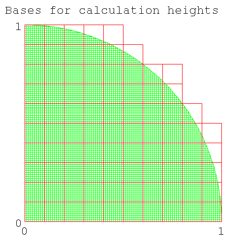
Number of column bases needed for height calculation for num_intervals=10
- Now calculate the volume of each column. Except for the top of the column, which is part of the surface of a sphere, the columns are square columns (with a square base). The volume under the curve has an upper bound, determined by the height of the highest corner of the spherical surface (this corner faces the center of the sphere) and a lower bound, determined by the height of the lowest corner of the spherical surface (this corner faces away from the center of the sphere).
- Now sum the volumes of all the slices. Do this with two loops, one inside the other. The inside loop integrates across each slice and returns the volume for the slice. The outer loop steps the calculation from front to back, each step calculating a new radius for the next slice (and hence the number of intervals in each slice) and summing the volumes from the inner loop.
-
How many iterations do you need for each loop?
Both ways are about the same amount of trouble.
- You could do a variable number of iterations for the inner loop, using a while loop. Since each quadrant has a different number of columns, the while conditional would test if you'd reached the end of the quadrant and then stop.
- You could do the same number of iteractions for the inner loop, using a for loop. The loop variable would range from 0.0..1.0*r. Since only 78% of the columns are inside the octant, 22% of them are outside and have a zero height. Calculating a zero height column for 22% of the columns isn't a big deal, if it simplifies the coding. However you'll still have to test if you're outside the octant before being able to declare a zero height.
| Note |
|---|---|
| End Lesson 30 | |
In this section the students prepared notes, diagrams, and tables for their presentation.
| Note | ||||||||||||||||
|---|---|---|---|---|---|---|---|---|---|---|---|---|---|---|---|---|---|
| |||||||||||||||||
The presentation should cover
- How numerical integration works: (you cut up an arbitary shape into many smallers objects - in this case a rectangle - whose area can be calculated. you can use my diagrams if you like.)
- The connection between the area of the quadrant as calculated by numerical integration and the value π.
- How you calculate the upper bound, the lower bound (show code, point out common numbers in both outputs)
- Show how one lot of code can calculate both upper and lower bounds
- Show the increase in precision in the value calculated, as the number of intervals is increased
- Show the (speed) optimisations that you tested, show the speed up from each. Discuss why you used some of these optimisations but not others.
- Show the output as a function of the number of intervals (value calculated, time taken).
- Estimate the upper bound for the error in the output.
- Discuss whether numerical integration is a useful method to calculate π (include time needed to calculate to 15, 100 decimal places).
- Compare speed of calculating π by numerical integration with other algorithms (Leibnitz-Gregory, Machin).
Arrays are useful data types in computer languages. You can expect all languages to have methods/functions for handling arrays. (Python has lists which are near enough to a 1-D array.) Here is an array of integers holding the temperature of each hour during the day. (In real life, this will be an array of reals rather than integers.)
temperature = [15,16,15,15,18,17,20,20,21,24,25,25,25,26,25,28,30,29,28,25,22,18,17,27] |
You can read/write elements of an array.
>>> temperature = [15,16,15,15,18,17,20,20,21,24,25,25,25,26,25,28,30,29,28,25,22,18,17,27] >>> print temperature[5] 17 |
Why wasn't the answer 18 [235] ? Write code to double the value held in temperature[5], and output it to the screen. Here's my code [236] . Let's find the max, min, average and temperature range for the day? This code is too long to do at the python prompt; write your code in a file temperature_array.py. Write array_max(), array_min(), array_average() and array_range() as functions taking an array argument and returning an int. (There are already functions in python for max(),min(). For practice, I want you to write your own functions that handle arrays. To find the min and max of two numbers, you can use the python functions min(),max(). Check, in your head, that you can write a max(),min(), before you go off an use the in-built python functions.)
Here's my code [237] and here's my output.
dennis:# ./temperature_array.py average: 21 min : 15 max : 30 range : 15 |
| Note |
|---|---|
| |
Computer languages don't have ways of addressing individual digits in numbers - you're only interested in the value of the number, not the digits that represent it in its decimal version.. However in most (all?) languages, strings are represented as an array of char and thus a programmer can individually address chars in a string. Programs dealing with text need to be able to search for substrings, change capitalisation, change word separators (e.g. ,:;), and reorder words.
>>> my_name="Simpson, Homer" >>> print my_name[3] p >>> for c in my_name: ... print c ... S i m p s o n , H o m e r >>> |
Why did this code print 'p' rather than 'm' for my_name[3]?
Using the string code above as a template, output a person's name in the reverse order. Here's my code [238] . Next output all occurrences of 's' (or a letter of your chosing) in a name as uppercase (use: string.upper()). Here's my code [239] .
| Note | |
|---|---|---|
I asked you to output the modified string, rather than modify the string in place and then output the modified string.
In python you can't modify individual char of a string
| ||
| Note |
|---|---|
| End Lesson 40 | |
A 2-D array could hold the height of ground at 1m intervals in an x,y grid, or the (r,g,b) value for each pixel (an element with a position in x,y) in a photograph. A 3-D array could hold the temperature of 1m cubes of the atmosphere; each element of the array would be indexed by (x,y,h).
Only a few languages (e.g. Fortran) have multidimensional arrays. Since python only has lists (a 1-D array), in python how would you store a 2-D array, e.g. the intensity of a black and white pixel in a photo [240] ? You could cut up the photo row or column-wise. As an example, here's a small image whose pixels can only have value 0,1
0 0 0 0 0 0 0 0 0 0 0 1 1 1 1 1 1 0 0 0 0 0 1 1 0 0 1 1 0 0 0 0 1 1 0 0 1 1 0 0 0 0 1 1 1 1 1 0 0 0 0 0 1 1 0 0 0 0 0 0 0 0 1 1 0 0 0 0 0 0 0 0 1 1 0 0 0 0 0 0 0 1 1 1 1 0 0 0 0 0 0 0 0 0 0 0 0 0 0 0 |
Here are the row-wise lists, followed by the image list
row9 = [0,0,0,0,0,0,0,0,0,0] row8 = [0,1,1,1,1,1,1,0,0,0] row7 = [0,0,1,1,0,0,1,1,0,0] row6 = [0,0,1,1,0,0,1,1,0,0] row5 = [0,0,1,1,1,1,1,0,0,0] row4 = [0,0,1,1,0,0,0,0,0,0] row3 = [0,0,1,1,0,0,0,0,0,0] row2 = [0,0,1,1,0,0,0,0,0,0] row1 = [0,1,1,1,1,0,0,0,0,0] row0 = [0,0,0,0,0,0,0,0,0,0] image = [row0,row1,row2,row3,row4,row5,row6,row7,row8,row9] |
Let's print the image. Swipe this code to array_image.py and run it.
#! /usr/bin/python # array_image.py # row_len=10 col_len=10 row9 = [0,0,0,0,0,0,0,0,0,0] row8 = [0,1,1,1,1,1,1,0,0,0] row7 = [0,0,1,1,0,0,1,1,0,0] row6 = [0,0,1,1,0,0,1,1,0,0] row5 = [0,0,1,1,1,1,1,0,0,0] row4 = [0,0,1,1,0,0,0,0,0,0] row3 = [0,0,1,1,0,0,0,0,0,0] row2 = [0,0,1,1,0,0,0,0,0,0] row1 = [0,1,1,1,1,0,0,0,0,0] row0 = [0,0,0,0,0,0,0,0,0,0] image = [row0,row1,row2,row3,row4,row5,row6,row7,row8,row9] #from top to bottom for y in range (col_len-1,-1,-1): #have to assemble whole line before printing #otherwise python puts an unrequested <cr> after each char line = "" #from left to right for x in range (0,row_len): if (image[y][x] == 1): line += "M" else: line += "." print line # array_image.py ------------------------------- |
Here's the output
# ./array_image.py .......... .MMMMMM... ..MM..MM.. ..MM..MM.. ..MMMMM... ..MM...... ..MM...... ..MM...... .MMMM..... .......... |
For the loop parameter y
- Why is the loop parameter run in the reverse order to the loop parameter for x (i.e. why is the 3rd parameter of range() -1)? Run the code with for y in range(0,col_len):
- Why is the 2nd parameter of range() -1 [241] ? Change the 2nd parameter to 0 and replace the "." in the output line by " ". Now look at the output. You'll be missing the last column but you can't tell.
- Why do I ouput a "." rather than a " "? [242]
In this code, what does the construct image[y][x] represent?
- image[] is a list.
- image[] has elements image[y].
- The element image[y] is itself a list (in this case, a row of pixels), so image[y] is a list of pixels.
- image[y] is a list (of pixels). The xth element of image[y] is image[y][x], a pixel.
Much of scientific computing is operations on large arrays. In a multitasking operating system, some other code could be running at the same time, and in the middle of your code allocating memory for the rows, someone else's cookie recipe code could run, putting the recipe in between two of the rows of your image. The memory for the rows of the image will not be contiguous. Access to your image array will be slow as the computer has to figure out where all the rows are each time it runs through the image. Its better to have the image stored as a continuous 1-D array. This requires the program (instead of python) to know where each row starts in the single array. This code is more complicated to write. If you have a small array and you aren't going to process it very often, then you should let python handle the indexing by using a list of lists. If you have a big array and it's accessed 1000's of times/sec as part of a numerical integration, then you bight the bullet and write code which indexes into a 1-D array (this is going to be more confusing than you might have first expected).
Copy array_image.py to array_image_2.py and rewrite the code to store the image in a single 1-D list. As in the previous code, make the bottom left corner of the image (x,y)=(0,0).
- Leave the row lists as they are (in global name space). Initialise the 1-D global variable image[] to the empty list. Keep the two global variables row_len, col_len. For the moment comment out the code that prints the image. You will later rewrite this code for the new format of image[]
-
write list fill_image() which takes no parameters,
reads the data from the various rown[] in global namespace,
and returns a 1-D list elements[]
containing all the elements of the rows.
-
Initialise a 1-D list elements[]
which you'll use to store the 100 elements.
Note It's convenient to name lists with a plural name, and name of each element with the singular e.g. each element of files[] is a file; each element of pixels[] is a pixel; each element of rows[] is a row. (Not everyone uses this convention.) -
Start with code to copy each column of some row
(any row e.g.row0) into elements[].
You iterate for each column in the row from the beginning of the row to the end of the row.
What code will you use to generate the loop parameter
(call your loop parameter col)
[243]
? Note which part of the line is associated with the number of columns
and which part of the line of code comes from the length of the row.
(You thought the fencepost problem was confusing.)
In python you add elements to a list using the list append() method.
elements.append(row[col])
-
Now you need to repeat this process for all rows.
Initialise rows[] at the top of fill_image[].
You need a loop parameter that assumes the value of each row (call your loop parameter row).rows = [row0,row1,row2,row3,row4,row5,row6,row7,row8,row9]
Now iterate over the all the rows, filling elements[].for row in rows:
- To confirm that the function works, inside the function code, print the contents of elements[] to the screen, (it should be a single list of 100 elements) then comment out the print statement.
- In main() call fill_image() and assign the returned list to image[].
-
Initialise a 1-D list elements[]
which you'll use to store the 100 elements.
- Write write_image(list pixels) by modifying the currently commented output code to accept the new (1-D) format of image[]. Check that your output image is the right size (has the right number of columns and rows).
Here's my code [244] .
| Note |
|---|---|
| End Lesson 41 | |
We're going to write code to do image transformations. Since we're now using a 1-D array, this is going to require translating between the index in the 1-D array (0-row_len*col_len)=(0-99), and the 2-D location of the element in (row,col) pairs. If you're fiendishly clever (in which case you won't be learning to program off a webpage) you can do this without making mistakes. The rest of us get into trouble here and we write a pair of functions to do it for us. With this pair of functions, we can treat a 1-D array as if it were a 2-D array.
| Note |
|---|---|
| When describing points in cartesian space, they are described by the pair x,y. But when describing arrays, they are normally described by row,col (i.e. the reverse order). The people who designed tables weren't the same people who designed the Cartesian coordinate system. Such is life (unfortunately). | |
Copy array_image_2.py to array_image_3.py. Add a function int row_col2index(row,col) which gives the index in the 1-D array for any row,col pair.
| Note |
|---|---|
| code which does simple transformations is often given a name like foo2bar (with the "2"). Though I think it ugly, it's a well accepted idiom (and I use it). | |
Here's my code for row_col2index() [245] .
| Warning |
|---|---|
| This function will happily accept parameters out of range (e.g.my_row<0, my_row>max_row) and depending on the values of the parameters may return an index that is in range (so you won't know you have a problem). If this code was going to be used in production, you will need to at least print out a message letting the user know that the parameters are out of range. | |
Include in main() some tests. While right now you can do a test by running print row_col2index(5,5) and confirming by eyeball that you got the right answer, this won't work in 6 months. Instead write array_image_tests() that contains groups of statements like
row = 0 col = 0 result = 0 if (row_col2index(row,col) == result): print "OK" else: print "expected %d, found %d" %(result, row_col2index(row,col)) |
Since you'll be doing the check many times, make the last 4 lines above into a function test_row_col2index(). Check that the test fails when it's supposed to. Here's my my first pass at code to test row_col2index() [246] (you'll make minor modifications shortly).
Write the complementary index2row_col(index) which turns an index into a row,col pair. index2row_col() returns two integers, but python (and most languages) can only return one item. What do you do in this case [247] ?
With a pair of names like index2row_col() and row_col2index() you (and anyone reading your code in 6 months) would reasonably expect these two functions to be the inverse of each other (i.e. if you run both of them, you'll be back where you started). However if you run index2row_col(row_col2index(row,col)), you will start with two separate integers and return a single list containing two integers. Anyone later reading your code will not be happy, when they finally figure out that the two functions aren't a pair of inverses. No-one forsees such problems; you just fix your code. What's the fix required to make these functions a pair of inverses [248] ? Fix your code (and the tests). Write a pair of tests to show that the two functions are inverses. Here's my version of the pixel to index position converters and the next iteration of their tests [249] .
Convert write_image() to use index2row_col(), row_col2index(). There is only one line changed. Here it is [250] . Make sure you understand the nesting of the different types of brackets. [] encloses a list; () encloses the parameters for a function.
Notice that the result from one test is the input for the other test. In that case there's no real reason to use the name result. It would be simpler to use a more descriptive name than result and to do both tests at once e.g.
#-------------------------------
def test_row_col2index(my_elements,my_index):
print "test_row_col2index"
if (row_col2index(my_elements) == my_index):
print "OK"
else:
print "expected = %d , found = %d" %(my_index, row_col2index(my_elements))
# test_row_col2index()----------
def test_index2row_col(my_index,my_elements):
print "test_index2row_col"
if (index2row_col(my_index) == my_elements):
print "OK"
else:
#could find how to format output of a list
#print "expected = %l , found = %l" %(my_elements, index2row_col(my_index))
print "expected = ", my_elements, " found = ", index2row_col(my_index)
# test_index2row_col()----------
def array_image_test():
print "array_image_test"
#points[row,col]
points = [0,0]
index = 0
test_row_col2index(points,index)
test_index2row_col(index,points)
.
.
|
result has become index or points (or a minor variation thereof).
Once you've convinced yourself that your code works, comment out the call to array_image_test().
Here's my code for array_image_3.py [251]
You might remember that one of the reasons for using a 1-D array to represent large 2-D arrays was speed. However function calls are slow, and we're going to be using functions each time we index or retreive a pixel at an index. In languages built for speed, these one-line function calls will be in-lined, i.e. the code for the function will be written directly into the code (instead of making the function call) and no function call will be made. This is done with a MACRO or an in-line compiler directive.
| Note |
|---|---|
| End Lesson 42 | |
Our code is filled with lines like
for col in range (0, row_len) . . for row in range (0, col_len) |
Mixing row and col in the same line like this is confusing and you'll get it wrong eventually (the variable col runs from 0 to row_len???; there would be less chance of a mistake if col went from 0 to some string with col in it). Although I'm used to this convention and originally wrote the code for this section using it, here's a better convention (I made a mistake in a later version of array_image.py and took at least a week to find it).
max_col=row_len max_row=col_len for col in range (0, max_col) . . for row in range (0, max_row) |
In case you're wondering, you can always think of a better way of doing it and you wind up rewriting your code a lot. Initially your code gets longer and longer and then it starts to get shorter. Copy array_image_3.py to array_image_4.py and change your code to use the new convention. Here's my code [252] .
For this section on arrays we're only interested in a square array (an image). The code has lines of code with parameters max_col or max_row (originally row_len, col_len). Of course we've thought carefully about which one to use, but since these two variables have the same value, we won't know if we got it wrong. You either have to document each function, saying that you don't have a clue whether you're using the correct variable, and that your code will only work for square arrays, or you can test your code. To test we need a rectangular array.
Copy array_image_4.py to array_image_5.py and put the code below into your global section.
| Note |
|---|---|
| You'll have to do minor surgery: rows[] has moved into the global section. Remove this code from fill_image(). | |
We use a conditional to determine which array is presented to the code. (This conditional is a bit of quick and dirty programming. If we were doing it properly, we'd pass the name of the array as an argument to a function. We're only writing this piece of code for a check, so it doesn't have to look great.)
# initialise global variables #large image image_large = [] row9 = [0,0,0,0,0,0,0,0,0,0] row8 = [0,1,1,1,1,1,1,0,0,0] row7 = [0,0,1,1,0,0,1,1,0,0] row6 = [0,0,1,1,0,0,1,1,0,0] row5 = [0,0,1,1,1,1,1,0,0,0] row4 = [0,0,1,1,0,0,0,0,0,0] row3 = [0,0,1,1,0,0,0,0,0,0] row2 = [0,0,1,1,0,0,0,0,0,0] row1 = [0,1,1,1,1,0,0,0,0,0] row0 = [0,0,0,0,0,0,0,0,0,0] rows_large = [row0,row1,row2,row3,row4,row5,row6,row7,row8,row9] #here's a line of code that assigns the dimensions of this array #for the large image, dimensions_large is [10,10] dimensions_large = [len(rows_large),len(rows_large[0])] #print dimensions_large #small image - a rectangular (rather than square) "y" with serifs. image_small = [] row_small_4 = [1,1,0,0,1,1] row_small_3 = [0,1,0,0,1,0] row_small_2 = [0,0,1,1,0,0] row_small_1 = [0,1,0,0,0,0] row_small_0 = [1,1,0,0,0,0] rows_small = [row_small_0,row_small_1,row_small_2,row_small_3,row_small_4] #use the same code as above to give the actual value of dimensions_small[] dimensions_small = [len(rows_small),len(rows_small[0])] #print dimensions_small #chose image to work on image_to_use = "large" # a string, allowed values - "large" or "small" if (image_to_use == "large" ): dimensions = dimensions_large rows = rows_large image = image_large else: dimensions = dimensions_small rows = rows_small image = image_small max_col = dimensions[1] max_row = dimensions[0] |
By assigning image_to_use = "large", this code is functionally identical to the previous code. Run it to check that it runs as before.
| Note | ||
|---|---|---|---|
In python when you assign values of primitive data types to a variable name, the variable is an independant copy of the original. Here b is an independant piece of memory: you can manipulate a and b independantly.
In python, all non-primitive data types are objects (which I've carefully ignored for the sake of simplicity). With objects, assignment makes an alias.
b is another name for a; there is no new piece of memory allocated for b. Why doesn't the interpreter/compiler make a copy rather than an alias? The simple answer is that figuring out code that will copy an arbitary object, which could itself be composed of other objects, each of which has primitive data types, is difficult. When you learn OOP, one of the first things you'll do is to write code to copy a particular object. You will see that generalisation of the process is not simple. One would think that since the compiler/interpreter has the definition of the object, that it should be able to copy any object. In principle this is true, but noone has written the code to copy arbitary objects; perhaps in a decade this will be a part of OOP. | |||
The code above makes dimensions, rows, image as aliases. In this section, you aren't going to be getting into any trouble because of this convention, but when you get to object oriented programming, you'll need to know the restrictions this imposes, so this is a good moment to alert you to the difference between a copy and an alias.
If you change the code to use the rectangular image, should your tests still work [253] ? Check that your code runs with the rectangular image as input. Here's my output
dennis:# ./array_image_5.py MM..MM .M..M. ..MM.. .M.... MM.... |
Since the code does produce the rectangular image, does this mean that you have chosen the correct places for max_row, max_col [254] ?
Producing the correct image doesn't prove that you have it right, but it's a good indication. For a quick check, change a few occurences of max_col, max_row to the other parameter name. Run the code again and look at the output; it should be wrong. If you do enough tests (changing max_row, max_col) and get corrupt images, most people will accept that your code is right. If you're an experienced programmer, then the simple check of showing that the code works with a rectangular array is good enough. Rarely in computing do you ever prove (in the mathematical sense) that your code is right. If you don't get into any further trouble down the line with your code, you probably have it right.
However this sort of check is handwaving and handwaving is OK if you're just having fun. If you're programming for real, you need tests at each stage that the code is working; tests that can be rerun in the far distant future when things have come unstuck and someone has to figure out what went wrong. You don't want to kill some otherwise healthy patient plugged into your heart monitor. Change array_image_test() to use the global variable image_to_use to add a set of tests for the rectangular image. Include tests that should fail. Here's my array_image_5.py [255] . Note I've made the output from the tests more informative (and shown how to print a list in test_row_col2index() and test_index2row_col()).
Shortly we'll do some transformations on the image: rotations and inversions, but first some theory. Pixels have integer positions. When a square image is rotated by a multiple of 90° or inverted, each pixel has only one place to go: there is a one-to-one mapping of source and destination. However if the image is rotated by any other angle (say 17°), the operations involve real (rather than integer) arithmetic and the location of the target pixel doesn't sit exactly in a pixel location on the integer pixel frame. In the early days of computer graphics, you would put the transformed pixel into the nearest pixel in the target grid. Sometimes two source pixels would land in the same target pixel (the last value entered being the one you'd see), while the adjacent pixel would get nothing and be blank (which might be rendered as black, white, grey or green, depending on the code). If you wanted to rotate the pixel set by 34° and you did 2 consecutive 17° rotations, another set of blank pixels would appear. After a few rotations, the picture would be a mess. Out of this computer graphics coders decided
- When doing multiple transformations; keep track of where you are and do the transformation from the initial orientation, rather than multiple incremental rotations. Thus any image displayed would only have been through one mathematical transformation.
- Rather than calculating the target location from the source location, instead for each target location, find a source location. Normally you'd look at the original pixel and work out where it should go. In graphics you do the inverse; for any target pixel, find the pixel which would produce it. You will still get image degradation; two adjacent pixels in the target will have come from the same source pixel, but rarely will the viewer notice this. This way you won't have any blank (black/white/grey/green) pixels.
We're only going to be doing operations which involve a one-to-one mapping of source and target pixels, so we won't have any of these problems. However since you're doing graphics, we'll code it up the way graphics programmers do it, starting with the target pixel and finding the corresponding source pixel.
| Note |
|---|---|
| End Lesson 43 | |
To invert the image, you'll need a new list to write the image into. Inside your invert function, you'll need to write elements (each is a pixel) to a new list. Here's two ways of doing creating a list and writing to it.
-
create an empty list,
fill it will anything to make it the right size,
then assign values to each element in any order.
inverted_pixels = [] #create the (empty, ie zero length) target list for i in range (0,max_col*max_row): inverted_pixels[i]= -1 #fill the list with an invalid pixel value, #allowing later checking for pixels #that haven't been assigned. #list now has max_col*max_row elements #fill list with pixels (in any order) pixel_index=5 #pixel location pixel_value=1 #pixel value inverted_pixel(pixel_index) = pixel_value #assign pixel element.
Note There is a list.insert(position, value). The element(s) starting at position all get moved along one place thus changing the position of elements already in place. -
create an empty list, fill from start to end of list, by appending elements to list
(this requires you to fill the output list in order).
inverted_pixels = [] #create the (empty, ie zero length) target list #fill list with pixel in order, from index=0 to index=last_member for i in range(0,max_row*max_col): inverted_pixels.append(pixel_value) #Append pixel to end of list #There is no "i" parameter, since there's only one end of list. #This requires doing operations in the order #of the index for the target list. #The length of the list grows by 1 for each append.
Either of these two methods can be used for your code. My code will use the first method as coding is simpler, when you can add elements in any order. As well it's the method used in C where arrays are not objects, but a slice of easy to access memory. Here's how you'd fill pixels in an array in a language like C or Fortran. Elements can be assigned to the array in any order.
int inverted_pixels[max_col*max_row] #create a list of correct size, #filled with random garbage #(whatever was in the memory #when it was allocated to the array) #fill list with pixels (in any order) pixel_index=5 #pixel location pixel_value=1 #pixel value inverted_pixel(pixel_index) = pixel_value #assign pixel element. |
Now let's look at the transformation needed to invert an image. If a pixel is in row y in the original image, and you're inverting the image top-to-bottom, what row in the output image, will the pixel wind up in [256] ? How about for columns [257] ?
If you were looping over the input rows, finding the pixel value and then looking for the location of the output pixel, you'd do this
for input_row in range(0,max_row): #do something with input row for input_column in range(0,max_col): #the arguments for row_col2index() are known, #they're the loop counters input_row and input_column value=input_list[row_col2index([input_row,input_col])] #We don't know the output [row,col] yet output_row = max_row -1 -input_row output_col = input_col output_list[row_col2index([output_row,output_col])] = value |
input_row will loop 0->9 and as a result output_row will loop from 9->0.
However we're doing graphics, so we have to loop over the output rows to make sure we fill them all. Write the code to instead loop over the output rows [258] ? This may seem a lot of complicated book work, when many people could write this code without functions like row_col2index() and without explicit formulae for converting the input row to the output row, but in 6 months, no-one will be able to read the code, not even you.
Copy array_image_5.py to array_image_6.py. Add code for list invert_top_to_bottom(list pixels), which takes an image[] and returns an image[] which is flipped top-to-bottom.
Output the inverted image in main() using write_image(). Here's my initial invert_top_to_bottom() [259] and here's my output showing the original and the flipped image.
pip# ./array_image_6.py .......... .MMMMMM... ..MM..MM.. ..MM..MM.. ..MMMMM... ..MM...... ..MM...... ..MM...... .MMMM..... .......... .......... .MMMM..... ..MM...... ..MM...... ..MM...... ..MMMMM... ..MM..MM.. ..MM..MM.. .MMMMMM... .......... |
Here's the top of the two nested loops. The transform here is easy to read.
for output_row in range (0, max_row): for output_col in range(0,max_col): #calculate the input [row,col] which maps to this output pixel #originally had max_col instead of max_row. It took almost a week to find it input_row = max_row -1 -output_row input_col = output_col |
But what's the sloppy programming [260] ?
The use of [row,col] in the code makes it hard to read. Here's more readable code - it at least removes one level of brackets.
#old code
pixel = pixels[row_col2index([input_row,input_col])]
inverted_pixels[row_col2index([output_row,output_col])] = pixel
#new code
#to make things easier to read
input_coords = [input_row, input_col]
output_coords = [output_row,output_col]
pixel = pixels[row_col2index(input_coords)]
inverted_pixels[row_col2index(output_coords)] = pixel
|
This adds a few extra lines of code, and presumably will slow down the code by a very small amount, but in the trade off of speed and maintainability, maintainability always wins.
Now that you've added -1 as the value for an unassigned pixel (in invert_top_to_bottom(pixels)), modify write_image() to output a char that you'll recognise as an error (e.g. "x") whenever it encounters an uninitialised pixel. Test that it works by running write_image() on an image containing unassigned pixels. (Hint: you generate an image with all unassigned pixels in invert_top_to_bottom(pixels)). Here's my modification to write_image [261] and here's my array_image_6.py with all the modifications above. [262] and here's my output, including the array of unassigned pixels
dennis: ./array_image_6.py .......... .MMMMMM... ..MM..MM.. ..MM..MM.. ..MMMMM... ..MM...... ..MM...... ..MM...... .MMMM..... .......... xxxxxxxxxx xxxxxxxxxx xxxxxxxxxx xxxxxxxxxx xxxxxxxxxx xxxxxxxxxx xxxxxxxxxx xxxxxxxxxx xxxxxxxxxx xxxxxxxxxx .......... .MMMM..... ..MM...... ..MM...... ..MM...... ..MMMMM... ..MM..MM.. ..MM..MM.. .MMMMMM... .......... |
Make sure your code runs on the rectangular image too.
All multidimensional arrays (in all languages) are stored as a 1-D array in the computer's memory. Memory accesses are faster if memory locations are accessed sequentially. The computer hardware fetchs a cache line (usually 4 to 8 words) in one swipe, even if you only want one byte. For a row with 10 integers, a fetch of the 0th integer will also retrieve the next 3 or 7 integers. Depending on the hardware and compiler optimisations, if you are moving through a large array, the computer might realise that you're streaming and do multiple pre-fetches. Let's say you write your 1-D array so that it looks like this
row col memory_location 0 0 0 0 1 1 0 2 2 0 3 3 1 0 4 1 1 5 1 2 6 1 3 7 . . 3 0 12 3 1 13 3 2 14 3 3 15 |
Now if you access each column in row 1 (at memory locations 4..7) then the computer can retrieve them all in one fetch. If instead you retrieve all rows for colum 1 (at memory locations 1,5,9,13), the computer will retrieve them in 4 fetches. In array intensive code, designed for speed (python is not designed for speed), you are expected to write your code to take advantage of the hardware's ability to fetch adjacent memory. You can't always do this; sometimes you read in column order and write in row order and you'll always have to wait for the one that's written in the wrong order. If an array has to be accessed many times in the wrong order, you rewrite the array (swapping columns and rows), do your operations and then write it back to the original format. The cost of the two extra writes can be made up by the savings in time from reading the memory in sequential order.
| Note |
|---|---|
| I couldn't find numbers on the internet, but I remember that having the row/column order wrong slows the program by a factor of about 4, enough to be obvious to anyone running the code People running code written the wrong way can often spot the problem straight off; they know how big the arrays are and how long it should take. It is just appalls me that code like this is released to users. | |
You access the array in nested loops, with the outer loop variable being one of row or column and the inner loop variable being the other variable (column or loop). You control the access pattern in 1-D memory by choosing the variable to control the outer loop and the variable to control the inner loop. Looking rows[] in the global namespace and its use in write_image(); figure out whether the elements of a row are adjacent in memory or whether the elements of a column are adjacent [263] .
Because of the way the initial array was written, for fast access to the elements of the array, you pick a row and walk along the columns.
| Note |
|---|---|
| This was set as homework. | |
Let's try another transformation. Copy array_image_6.py to array_image_7.py. Add list invert_left_to_right(list pixels) which flips pixels left to right, and code in main() to show the flipped image. Here's my invert_left_to_right() [264] and here's my code in main() [265] .
When you multiply numbers, you get the same result, no matter which order you multiply the numbers.
3*2=2*3=6 |
In mathematical terms, 2 and 3 commute under the operation of multiplication. In conversation you say "multiplication is a commutative operator". Is addition a commutative operation [266] ?
Do the two image inversions invert_top_to_bottom(), invert_left_to_right() commute (i.e. does it matter what order you do them)? (You should be able to get the answer in your head.) Look at the output image after applying both operations in different order. If you wanted the computer to do the test (rather than you looking the two images), how would you get the computer to check whether the outputs were the same? Here's my code [267] .
We conclude that the two inverting operations (top-to-bottom, left-to-right) commute. We'll return to commutative operations shortly, and we'll see some operations don't commute.
As well, the two inverting operators each are their own inverse. If you flip top to bottom twice you restore the original image. What number is its own inverse under the operation of multiplication?
let A be self inverse under multiplication let z be any real number then z = A*A*z in which case A^2 = 1 A = +/- 1 |
The numbers 1 and -1 are self inverses under multiplication. What number(s) are self inverses under addition [268] ? Operations which are self inverse are relatively uncommon. In our day-to-day world, some light switches operate as their own inverse: each time you press them, the light changes state (on/off). If you press it twice, the light returns to its original state.
| Note |
|---|---|
| End Lesson 44 | |
| Note |
|---|---|
| For the python class, we're only going to do rotations of multiples of 90°. | |
In the Cartesian coordinate system (http://en.wikipedia.org/wiki/Cartesian_coordinate_system), the direction of +ve rotation is anticlockwise. Thus a vector (http://en.wikipedia.org/wiki/Euclidean_vector) from the origin (0,0) along the +ve x-axis, if rotated 90° would point along the +ve y-axis. The cartesian system divides the plane into 4 quadrants (see Fig 3 on the wiki page for the Cartesian coordinate system).
A square image like ours, with lower left corner=(0,0) and upper right corner=(9,9) sits in the first quadrant. A rotation of the image is done by rotating the vector to each pixel about the origin. If the image were rotated by +90° the rotated image would sit in the 2nd quadrant (the pixel that was at (0,0) is still closest to the origin, while the pixel that was at (9,9) would still be furthest from the origin, but all in the 2nd quadrant); if rotated by +(or -)180° it would sit in the 3rd quadrant; if rotated by 270° or -90°, it would sit in the 4th quadrant.
There are only 4 different rotations by multiples of 90°: 0,90,180 and 270°. Adding or subtracting 360° does not change the rotation (540°==180°). Any other +ve or -ve rotation can be shifted by multiples of 360° to one of these 4 angles. If we're given a rotation of -270°, how could we change the rotation to what I'm calling normal form [269] ? If we're given a rotation of 540°, how could we reduce it to normal form [270] ? What happens if you modulo a +ve number, a -ve number (try -540° 450°)?
Copy array_image_7.py to array_image_8.py. Add int normalise_angle(int) to change an arbitary angle to normal form and give an error message if it isn't a multiple of 90° Here's my code [271] and here's my test code in main() [272] and here's my output [273] .
| Note |
|---|---|
| Normally on an error, you want the program to exit or to return an invalid number. Since valid answers are +ve, on an error, I have the function return -1, which the calling code can detect and handle. Since we aren't handling errors (a more complicated topic, that we don't handle in this course), make sure your code only valid input i.e. multiples of 90° | |
To array_image_8.py add list rotate(list pixels, int angle). First parse the rotation angle and determine the number of 90° rotations (it will be 0,1,2 or 3). Setup a stub loop which does these rotations.
| Note |
|---|---|
| a stub is a piece of code that does nothing (or very little e.g. prints "hello from stub"), which accepts the calling parameters and, if required, returns a dummy variable to the calling function. A stub lets the whole program to run, allowing you to defer filling the contents of the stub later. Stubs are used extensively in top-down programming. | |
For the stub code, use something diagnostic (e.g. print or print angle). Check that you get the expected number of lines output to the screen (how many rotations are you going to do for rotate(0)?).
Now we want the operation that rotates a set of pixels by 90° about the center of the image. We do this in two steps
-
First we'll rotate the pixel (actually the vector from the origin to the pixel) about the origin
(putting the pixel into the 2nd quadrant, where the column indices will all be -ve).
Note "rotating a pixel" means rotating the line joining it to the origin, about the origin; not rotating the pixel about its center. -
we translate the pixel horizontally back into the first quadrant
(i.e. we translate the center of the pixel).
Note defn: translate - move whole object (image, point, vector) in a straight line without rotating it.
We rotate the pixel by the following operation
x_new = cos(A)*x_orig - sin(A)*y_orig y_new = sin(A)*x_orig + cos(A)*y_orig |
| Note |
|---|---|
| The angle argument in python (and in calculus and in most math) is in radians, not degrees. For info on python's trig functions and using radians, see trigonometry. | |
This formula is normally written as a (see Rotation matrix)
|x_new| |cos(A) -sin(A)| |x_orig| | | = | | | | |y_new| |sin(A) cos(A) | |y_orig| |
If you want to rotate your image by an angle which is not a multiple of 90°, you'd use these functions. For A=90° the formula reduces to
x_new = -y_orig y_new = x_orig |
Confirm that this formula works for points on a circle with center (0,0), radius 1, which lie on the x and y axes (these points are at (1,0), (0,1), (-1,0), (0,-1)). When written using row,col this becomes
output_col = -input_row output_row = input_col |
After rotation, our pixel now is in the 2nd quadrant. What do you have to do to pixel(x,y) to translate it back to the 1st quadrant [274] ? What are the formulae for output_col, output_row for producing a rotated image back in the first quadrant (i.e. for doing both steps; rotation by 90° followed by tanslation) [275] ?
Add code to array_image_8.py to rotate the image by 90° (don't write the code to loop multiple times just yet). Then to rotate multiple times (e.g. 180°), from main(), use multiple lines of the same code to feed the resulting image back to rotate(). When that works add the loop code to rotate() to handle multiple rotations of 90°. and pass the rotation angle to rotate() as an argument from main(). Don't worry about the nesting of the column/row loops just yet (to speed up memory access). This is a fairly complicated piece of code. See how far you get without my help. If you're stuck here's how I did it [276] , here's my rotate() [277] , here's my main() [278] and here's my output [279] .
What to do about the order of nesting of the loops? It turns out that when rotating by 90° if you sweep the input array by rows, you sweep the output array by columns. There isn't anything you can do: one of the arrays will be swept in the wrong order and rotation will be slow. Such is life.
For reference here's my array_image_8.py [280]
In my implementation of rotate(list), to rotate by 270°, I rotate 3 times by 90°. Obviously this is slower than rotating once by -90°. Why is speed not important here, when I'm going to all the trouble of emulating a 2-D array with a 1-D array, to get a speed advantage?
- If this was final production code and speed was important, you would have 3 different pieces of code for +90°, +180° and +270° rotations.
- I can get the functionality I want with one piece of code and have it running in shorter time from the start of programming.
- You would leave it this way if maintenance was your most important goal. An important design goal is to minimise the number of paths through your code. If the logical flow can go in two directions, depending on the case being analysed, and if you find a bug in one branch, it's possible that the same bug will be in the other branch. It's also likely that when doing maintenance, you'll forget to update the other branch(es), or you mightn't know the other branch exists (it may be in another module). Having only one function to do the rotation means that any updates will occur to all three functionalities at the same time.
- I'm taking advantage of new situations to show different aspects of writing code (i.e. I'm doing it for teaching purposes).
When/if you split the 3 functionalities into 3 pieces of code, it would be best to leave all 3 functionalites in one function, so there's more chance they will all be updated at once. You would have code up the top of the function, which branched according to the argument to rotate().
What should your code do to the rectangular image. After you've got an answer, run your code. Make sure you can explain what' happening. [281]
The two operations, flip left-right and top-bottom, commute. We're so used to real numbers commuting under multiplication and addition, that it's a bit of a surprise (to some of us), to find that most operations do not commute. Numbers do not commute under subtraction
3 - 2 != 2 - 3 |
If the operation of putting on your socks is called SOCK and the operation of putting on your shoes is called SHOE, then the operation of putting on your socks and shoes is written as SHOE*SOCK.
| Note | |
|---|---|---|
The event would formally be described as
| ||
| Note |
|---|---|
| The "*" is not the multiply operation. It's a typographic convention saying "do SOCK, then do SHOE". It could be written in many ways e.g. SHOE.SOCK or [SHOE][SOCK]. The "*" is to stop the typesetting from putting a line break between the two operators and to make it easier to see where one operator starts and then next one finishes. | |
The operations of putting on your socks and putting on your shoes do not commute. If you do these operations in the reverse order, you get a different result.
Let's see whether a 90° rotation and flipping top_to_bottom commute (try it in your head or with pencil and paper first). Copy array_image_8.py to array_image_9.py. Add code to main() to output the images and have the computer check whether the results are the same. Here's my code in main()
#main()
image = fill_image()
image_rotated_90_then_flipped_vertically = invert_top_to_bottom(rotate(image,90))
write_image(image_rotated_90_then_flipped_vertically)
print
image_flipped_vertically_then_rotated_90 = rotate(invert_top_to_bottom(image),90)
write_image(image_flipped_vertically_then_rotated_90)
print
if (image_rotated_90_then_flipped_vertically == image_flipped_vertically_then_rotated_90):
print "they're the same"
else:
print "they're different"
|
and here's my output
dennis:/src/da/python_class/class_code# ./array_image_9.py .......... .M......M. .MMMMMMMM. .MMMMMMMM. .M..M...M. .M..M..... .MMMM..... ..MM...... .......... .......... .......... .......... ......MM.. .....MMMM. .....M..M. .M...M..M. .MMMMMMMM. .MMMMMMMM. .M......M. .......... they're different |
What about inverse of the operation of two non-commuting operators? Let's find the inverse of SHOE*SOCK? If the inverse of SOCK is written SOCK-1 (i.e. taking off your socks) and the inverse of SHOE is written SHOE-1, then what is the inverse of SHOE*SOCK (think of what you have to do to get your shoes and socks off)?
X = (SHOE*SOCK)^-1 X = SOCK^-1*SHOE^-1 |
First you take your shoes off, then you take your socks off. If you want to invert the operation of a pair of non-commuting operators, you have to perform the inversions in the reverse order as well.
Let's invert the result of the two operations we've just done on the image. For each of the rotate and flipping operations, find the inverse operation. If
- rotate(image,90) is represented by R(90)
- invert_top_to_bottom(image) is represented by I
then what is the inverse of rotate(image,90), of invert_top_to_bottom(image) [282] ? Applying the rule for inverting a pair of non-commuting operators (you apply the inverse operations in reverse order), we get
(I*R(90))^-1 = R(90)^-1*I^-1 = R(-90)*I. |
Let's look at the mathematical notation for the operation of inverting the original two operations.
first two operations = I*R(90) proposed inversion = R(-90)*I operation which should restore original image = R(-90)*I*I*R(90) but I is its own inverse so I*I = 1 then result = R(-90)*R(90) but R(-90) and R(90) are inverses then result = 1 |
We're back to our original image.
Here's my code in main() [283] and here's my output [284] .
Assume the computer is doing something like a Rubic's Cube. Are there different ways to get to the same result? Can we do the equivalent of one inversion and one rotation using another pair of operations, to get the same image? Do it in your head and then confirm your choice with the computer. Here's my result (using the abbreviations T = invert_top_to_bottom(), L = invert_left_to_right()) [285] . Why is this so? In the general case, we can't stack operators on the right hand side, only the left (where we operate on an image).
To prove: T*R(90) = L*R(-90) operate on both sides by L. L*T*R(90) = L*L*R(-90) we know that L*L = 1 #L is its own inverse, L*T*R(90) = R(-90) and by inspection L*T = R(180) #yes we could prove this if we had to. thus R(180)*R(90) = R(-90) but R operations are additive, so R(180)*R(90) = R(270) R(270) = R(-90) we can normalise R(-90) to R(270) R(270) = R(270) QED |
We've got one more thing to do in array_image_9.py.
| Note |
|---|---|
| End Lesson 45 | |
In our code we've got a few lines like
max_row = dimensions[0] max_col = dimensions[1] |
While you and I know what element [0] and element [1] are in element_list[], no-one else is going to know and you won't in 6 months either. How long/large is element_list[]? If you guess that it's a set of coords, are the coords in the order x,y or row,col (if you guess wrong, all your code will work, but when it calls someone else's code, the Shuttle is going to blow up).
A programming convention is to use constants (variables in global namespace which you agree not to change), whose name are distinctive and recognisable to a programmer, that hold these values. These variables are usually all caps and you never attempt to change them (these can be called "literal constants"). The above code would become
#global namespace ROW_INDEX = 0 #for coordinates COL_INDEX = 1 . . . #inside function max_row = dimensions[ROW_INDEX] max_col = dimensions[COL_INDEX] |
ROW_INDEX, COL_INDEX are just another glocal variable to python, and python will quite happily change them if you ask it to, but by the all caps convention, you and any other coders who look at the code agree not to change the values.
| Note | |
|---|---|---|
In other languages you declare these names to be constants and the languge will not let you change the values.
This is a better construct e.g.
| ||
Change the numerical values to literal constants. Here's my array_image_9.py [286] .
Rotating rectangular images by multiples of 90° is a routine operation in photo/image manipulation software packages. To rotate the rectangular image by 90°, you have to swap the values of max_row, max_col.
| Note | |
|---|---|---|
It would be better to put the pair max_row, max_col
through a rotation process as is done for a pixel,
but we don't have to get everything perfect here,
so we'll just swap the values.
The usual way of swapping two variables is
| ||
The problem with this approach to changing the array dimensions of the array is that max_row, max_col are global.
| Note |
|---|---|
A global variable is a variable in global namespace that you expect to be able to change (i.e. it's variable). Global variables are generally frowned upon (see global variable http://en.wikipedia.org/wiki/Global_variable). Global variables are allowed in certain situations, e.g. while you're developing your code, to make life easier. There aren't global constants in python, so you make them up. A global constant (or just "constant") is a global variable that you signal somehow (e.g.) by giving it a name in all caps), to all following programmers, that you won't change it. Global constants are initialised at the start of the program, they never change and are used to control the execution of the program. Global constants are just fine in all languages. In some languages (C++, Java), the compiler will give error messages if your code attempts to change them. | |
Some languages allow you to change global variables at will; other languages (C++, Java) do not allow you to change global variables; python allows you to change global variables using an "are you sure" type of instruction. Swipe and run this code (call it global.py)
#!/usr/bin/python #global.py #illustrates global variables #from a posting by rshaw on linuxquestions status = 1 #---------------------------------- def changetext(): status = -1 #status is local variable, not the global variable print "changetext: status", status #print local variable # changetext----------------------- def changetext_2(): print "changetext_2: status", status #global variable #local variable, will get a warning because of following "global status" command status = -2 print "changetext_2: status", status global status #all subsequent operations use the global variable status status = -1 print "changetext_2: status", status # changetext----------------------- #main() print "status", status #global variable changetext() #doesn't change global variable print "status after changetext", status #global variable changetext_2() print "status after changetext_2", status #changed global variable #----------------------- |
Here's my output (make sure you understand the effect of the command global status)
class_code # ./global.py ./global.py:16: SyntaxWarning: name 'status' is assigned to before global declaration def changetext_2(): status 1 changetext: status -1 status after changetext 1 changetext_2: status 1 changetext_2: status -2 changetext_2: status -1 status after changetext_2 -1 |
If you want to change a global variable in a function in python, you have to explicitely say so. If we wanted a quick and dirty piece of code to exchange max_row,max_col, we could change the global variables using the above method. However
- You need to learn to program without global variables. In exam situations you will loose marks for using them.
- In the review section for arrays review arrays I ask you to extend the code to simultaneously manipulate two images (e.g. inset a small image in the corner of a large image). There you will need two different sets of image dimensions. You will need sets of dimensions for each image being manipulated; i.e. your code needs to know ahead of time the number of images it will be dealing with. Again this is ugly.
The dimensions of the image have to accompany the image or we won't know how to draw it. Let's bight the bullet and pass the dimensions of the array/image as an extra parameter to all functions that have previously used the global values. (To keep down the number of parameters passed, pass the pair of numbers as a list of two elements.)
Copy array_image_9.py to array_image_10.py. Change row_col2index() so it accepts the extra parameter (the dimensions array). You will eventually have to change all the code which interfaces with the converter functions, but you only want to do it a function at a time, allowing you to fix mistakes as you go.
| Note |
|---|---|
| In an interpreted language, only the code in the executed path is seen by the interpreter. You can change the parameters for a function and the calls in the executed path, while leaving the other calls with the original parameters. By judicious choice of the executed path, you can change your code a little bit at a time. In a compiled language, all functions and calls to the functions must match, whether they're ever executed or not. In either case a programming editor will help the changeover. | |
Initially, do not run the code for testing these converter functions. Change the first function to call this converter (i.e. write_image()) and run it (and nothing else) from main(). To make the code more readable, I change all occurences of [row,col] to coords[] where coords=[row,col]. Check that the code works for the square and the rectangular image. Here's my row_col2index() [287] and here's the modified write_image() [288]
| Note |
|---|---|
| write_image() uses the (read only) global variables max_row, max_col to set the dimensions of the image it writes. What will happen when write_image() writes a rotated rectangular image [289] ? Using global variables is fine for the moment (Rome wasn't built in a day). You don't need to fix this till you start rotating rectangular images. | |
Move through the code changing functions to the new format (invert_top_to_bottom(), invert_left_to_right()).
| Note |
|---|---|
| I'm quite surprised to find that the highly useful converter function index2row_col() isn't used anywhere in the code. ;-) | |
Then do the test functions (some expressions will need the parameter dimensions twice). We now have the original code changed over to pass the dimensions of the array to the functions. We don't have any new functionality (we're just getting ready for it).
Now tackle rotate(), testing it first with a 90° rotation of the square image (i.e. without having to change the aspect of the target image). When you get to rotating the rectangular image, you'll find the problem mentioned above for write_image() which needs to know the dimensions of the image it is writing. Check that this is the problem by manually changing max_row,max_col for write_image() when it's writing the rotated rectangular image. Here's my rotate() [290] , here's my main() [291] and here's my output showing the original rectangular image and the (correctly) rotated copy. [292] .
We've now got working code (but only just). Here's the problem
Problem: The functions have access to both the pixels of the image and the dimensions of the image, so any functions called by other functions have access to both lots of data. However in main(), where write_image() sits, the dimensions of the image(s) are not available because, well, we decided not to use global variables. The problem is that we can't output an image with write_image() because it's at the top level of namespace and doesn't know the dimensions of the image.
What can we do about this?
- Could we move write_image() into the functions? Well possibly, it would be quite burdensome to do so. In our design, we have images in main() where we do things to them, like flip, rotate and write. Functions should be modular (have only one purpose) and you should be able to combine functions in arbitary order. To be required to move write_image() into one of the functions to get it to work, should be an alarm letting you know that you have a design problem.
Could we somehow associate the dimensions data with the pixels data, so that when write_image() is given the pixels, it can figure out the dimensions?
Computer programs need to keep track of related information about a single entity all the time. e.g. a photo downloaded from a digital camera, is accompanied by an EXIF header (http://en.wikipedia.org/wiki/Exchangeable_image_file_format) containing (among other things) the camera type, the exposure information and a thumbnail photo. An image then is not only the pixels, but almost anything the photographer wants to know about the photo and a thumbnail.
In a computer, related information is stored as a struct (structure, in procedural languages) or object (in OOP languages). If you wanted the exposure, you'd ask for image->exif->exposure. If you wanted the pixels, you'd ask for image->pixels[row,col]. Objects (in OOP) have attributes to do the same thing.
We haven't done structs yet (we'll meet them in C) so we can't use them. We're not doing any OOP till much later, so we can't use objects either.
How about we put the dimensions as an extra two elements into the pixel array (either at the beginning or end)? There's a couple of problems with this
- You would have to change row_col2index(), index2row_col(). Worse things could happen, but you have routines which have been well tested: they not only survive your tests, but they've survived, without any signs of distress, being beaten on by your subsequent additions to the program, not all of which worked (at first). You should not change working and tested code without a very good reason. If you need to change a functionality, instead encapsulate your unchanged working functionality so that it appears to the user in the required manner.
- Let's say you did change the structure of the pixels array. The code would need a conditional to decide if you were in the dimensions part of the array or in the pixels part of the array. This would be ugly. Sometimes code is ugly and there's no way around it, but ugly code is another indication of a design problem and shouldn't be ignored.
- In most languages (but not python) the elements of an array must be of the same type (e.g. all integer or all real or all strings). Right now the pixels and dimensions are integers. In a real image manipulation program the pixels will be 3 (or 4) integers representing R,G,B (or R,G,B, α). The dimensions might be the actual size of the image e.g. a real, 2.5 or a string "2.5cm". You should expect if your image_array code works, that someone will next want 3 color pixels and to rewrite the code in a language where all array elements are of the same type.
- This solution is unbelievably ugly. You may not see this yet, but after writing enough code, you'll recognize really bad ideas quickly.
What's the solution? How about you spend upto a few days thinking about this. If after a few days, you need a hint here's the method I got to work [293] .
Here's my solution: make pixels a list of lists.
PIXELS_INDEX=0 #for image DIMENSIONS_INDEX=1 . . pixels = [[],[]] #initialise an empty list of lists pixels[PIXELS_INDEX] = [] #initialise empty list of pixels; #you don't really need to do this, since it's already empty #but it makes clear what you're doing pixels[DIMENSIONS_INDEX] = [max_row,max_col] #initialise dimensions |
As above, change fill_image() and write_image() to handle the new variable and accept/return the correct parameters. Note the error messages you get when the code isn't right (they won't be terribly helpful) - you'll get the same errors as you work your way through the rest of the code. Do you have to change row_col2index() [294] ? Test with both images. Next change invert_top_to_bottom() and invert_left_to_right(). Then do index2row_col() the routines which test the converter functions and lastly rotate().
We're in the process of removing variables and code from global namespace. After converting your code to use local variables for the dimensions of the 2-D arrays, you can comment out (and later remove) the global namespace code that assigns values to max_row,max_col (and check that your code runs without them).
The images are in global namespace. I real life, arrays like rows_large[] would be read from a file. To save us the coding, we're going to allow the images to be in global namespace. You can input images by having statements like this
#This code is required to generate the 2D array. #Normally the 2D array would be generated outside this program #and we wouldn't see these next lines. row9 = [0,0,0,0,0,0,0,0,0,0] row8 = [0,1,1,1,1,1,1,0,0,0] row7 = [0,0,1,1,0,0,1,1,0,0] row6 = [0,0,1,1,0,0,1,1,0,0] row5 = [0,0,1,1,1,1,1,0,0,0] row4 = [0,0,1,1,0,0,0,0,0,0] row3 = [0,0,1,1,0,0,0,0,0,0] row2 = [0,0,1,1,0,0,0,0,0,0] row1 = [0,1,1,1,1,0,0,0,0,0] row0 = [0,0,0,0,0,0,0,0,0,0] #The variable we want is the 2D array rows_large[] rows_large = [row0,row1,row2,row3,row4,row5,row6,row7,row8,row9] |
in global namespace, but all other variables should go.
There are various forms of dimensions[] variables in global namespace. The functions should be able to figure these out from the 2-D image array. Change fill_image() to accept arrays like rows_large[] as a parameter and have the function determine dimensions from the 2-D array passed to it. Change fill_image() to use row_col2index() to construct the 1-D image array.
If you handed the code for fill_image() to a naive programmer, they wouldn't guess from the name that the function actually converts a 2-D array to our special format 1-D array. Give fill_image() a better name. I chose linearise_2D_image(). Put some documentation in the function, so that people will know what it does. Make sure that the understand the structure of the returned array.
Here's my linearise_2D_image() [295]
As is normal, the code has cruft from earlier stages, when we didn't know what the code was going to look like. Let's do some code clean up.
-
We have lines like this
This line with multiple occurences of points, dimensions is little hard to read. We could make dimensions part of an array containing both points and dimensions and the line would readif (points == index2row_col(row_col2index(points,dimensions),dimensions)):
This construct only occurs a few times and it's probably best to leave it as is. To change it in the manner described would require packing and unpacking arrays. It's possible as the code progresses to 3-color pixel etc, that we might need to deal with the (points,dimensions) construct in the future. We can't anticipate the future; let's wait till it happens.if (points == index2row_col(row_col2index(points))):
- There are comments about alternate ways of writing the code, which were inserted for didactic reasons. As always happens you try different ways of doing things and you leave old attempts buried in comments in case you need to go back. There'll be lots of commented print statements. Clean up the comments. Leave enough comments so that in 6 months you can figure out what the code is doing. It's a little hard to think of what you might forget/remember in 6 months, but as you accumulate code you'll start to get the idea of what you personally need; if in doubt, err on the side of leaving more comments in. No matter the state of your code, someone will always moan about the deficiency or the excess of comments. You'll never keep them happy: find a level you're happy with.
- In array_image_test() the path through the function is chosen by the variable image_to_use. This is a (so far necessary) kluge. The path through the function should be chosen by dimensions. Fix up this function.
Make the parameter names consistant:
(paraphrased from Steve Litt on the TriLUG mailing list). If you're sorting the score of people, in main() you'd call sort(people). The sort() can sort anything, not just people, so the declaration for the sort routine would be def sort(array). The function parameter should have some generic name to help the reader identify the types of algorithms likely to be used. If low level data types (e.g.coords, index are being passed from one function to another, then it's probably best to keep the name the same in the calling code and in the function.
The images in main() have names like image. When the image arrives in a function, it has the name pixels (array would be OK). I've used the same name dimensions for the calling parameter and for the argument to functions. For pixel coordinates, which go through several levels of calls, I've used different names (e.g. elements, points) in different functions: I've changed these all to a name like coords.
- The original images had names with big,small in them. While this was the obvious difference at the start, for the code the most important part was that the images were square or rectangular. Change the image names to rows_square,rows_rectangular.
Here's my array_image_10.py [296] and here's my output for the square image.
dennis:# ./array_image_10.py .......... .MMMMMM... ..MM..MM.. ..MM..MM.. ..MMMMM... ..MM...... ..MM...... ..MM...... .MMMM..... .......... .......... .MMMMMM... ..MM..MM.. ..MM..MM.. ..MMMMM... ..MM...... ..MM...... ..MM...... .MMMM..... .......... .......... .......... ..MM...... .MMMM..... .M..M..... .M..M...M. .MMMMMMMM. .MMMMMMMM. .M......M. .......... .......... .....MMMM. ......MM.. ......MM.. ......MM.. ...MMMMM.. ..MM..MM.. ..MM..MM.. ...MMMMMM. .......... .......... .M......M. .MMMMMMMM. .MMMMMMMM. .M...M..M. .....M..M. .....MMMM. ......MM.. .......... .......... |
and for the rectangular image
dennis:# ./array_image_10.py MM..MM .M..M. ..MM.. .M.... MM.... MM..MM .M..M. ..MM.. .M.... MM.... M.... MM... ..M.. ..M.. MM.MM M...M ....MM ....M. ..MM.. .M..M. MM..MM M...M MM.MM ..M.. ..M.. ...MM ....M |
Our code now has some reasonable functionality, is documented and tested, has no global variables and is ready to be handed off to someone else to peruse, use (or maintain). If you were writing a real image manipulation program, this would be a good proof of principle piece of code.
Say we have (3.14157, 3.14161) as the (lower,upper) bounds for π. To get a value for π we compare the digits one by one, till we get a mismatch giving the result π=3.141. Since strings are arrays, and there are functions to look at each char in a string, the simplest way of matching digits in a number, is to convert the number to a string and then march through the string retrieving each char, and test for a match to the corresponding digit in the other number.
But first we'll look at a few ways of finding matching digits in two numbers giving you practice with arrays.
Let's retrieve each digit as an integer.
Given the number 3.14157, what operator (and operation) would retrieve the digit 3 [297] ? Note: we want the value of the digit in a variable; the code print "%1d" %digit only shows that we're on track. Note: what if (number-remainder) returned 2.99999999? I couldn't find what the python function int() does in this case, but assuming it's like C, then the real will be truncated, giving 2 as the answer. Here's a fix (assumes we're only going to retreive the first digit each time, so adding any number slightly greater than 1.0 will do).
>>> digit = (number - remainder)*1.001 >>> print digit 3.003 >>> int_digit = int(digit) >>> print int_digit 3 |
Here's another way of doing it.
>>> number=3.15147 >>> int_number=int(number) >>> print int_number 3 >>> digits_in_lower_bounds = [] >>> digits_in_lower_bounds.append(int_number) >>> print digits_in_lower_bounds [3] |
How do we get the next digit? We put this code into a loop. Do we use a while or for loop? Whichever you choose, how do you terminate the loop? Write code, called turning_reals_into_digits.py that does the following.
-
initialises
- number which holds the real (give it some value typical of lower_bounds)
- number_of_digits the number of digits of number to extract (assume a 64 bit real). This is used to terminate the for loop. Could you use a while loop [298] ?
- digits_of_number[] a list to hold the digits in number.
- finds the first digit (stored in int_digit), using the above code and puts the value into digits_of_number[]. Output the contents of digits_of_number[] to the screen.
-
Next subtract int_digit from number
and shift all the digits in number one place to the left,
to give a value of number
from which you'll extract the next int_digit.
Note This shifting has the same problem with representation of reals as does the previous method. Each time you shift in the loop, you'll add rounding errors and errors due to the inability to exactly represent reals on a computer. (and in this case you can't multiply by 1.001.) Your only option to get a reasonable answer is to use a real with a sufficient number of bits to represent the number accurately enough for your purposes. - Put this code into a loop and extract all the digits from number, and output the contents of the list to the screen.
Here's my code [299] and here's the output.
pip:/src/da/python_class/class_code# ./turning_reals_into_digits.py 3.14157 3 1.4157 1 4.157 4 1.57 1 5.7 5 7.00000000002 7 1.95683469428e-10 0 1.95683469428e-09 0 1.95683469428e-08 0 1.95683469428e-07 0 1.95683469428e-06 0 1.95683469428e-05 0 0.000195683469428 0 0.00195683469428 0 0.0195683469428 0 0.195683469428 0 [3, 1, 4, 1, 5, 7, 0, 0, 0, 0, 0, 0, 0, 0, 0, 0] |
The trailing digits are 0's, because I used a truncated value for lower_bounds. The number could have rounded down, in which case the trailing digits would be all 9's.
Here's a better method to find the digits in a number, by turning the number into a string (an array of char). There are no rounding errors caused by multiplication by 10.
Here's a lower bound as a string.
>>> number = 3.14157 >>> str_number = str(number) >>> for c in str_number: ... print c ... 3 . 1 4 1 5 7 |
The function len() returns the length of a string. Use the result of the len() function to setup a loop which walks through a string (in this case the string representation of a number), outputting each char (in this case a decimal digit). Here's my code [300] .
Is there a fencepost problem in the number of times you iterate through the loop? How many times will the loop execute if it uses range(0,len(string_1)): to generate the loop parameter? (i.e. will the loop fall off the end of the string; will the code stop one place too soon?) [301]
You'll use this string comparison code for the last step of the numerical integration of π.
This section is set pieces of information that I keep referring to. Initially each piece was in a relevant section, but I kept reordering sections, and I'd wind up talking about list[] before I explained how they're used.
Here's a documentation template for a function
""" name: fencepost(d) author: Fred Flintstone (C) 2008 license: GPL v3 parameters: d: int or string; length of fence returns: number of fence posts, int modules: imports math method: assumes a distance of 10 between fence posts. number of fenceposts=(length of fence/10)+1 """ |
Here's a code fragment that generates a random number
>>> import random >>> random.randint(0,10) 0 >>> random.randint(0,10) 6 |
random is a module (code that's not part of the base python code, but can be imported to add extra functionality). In the above example, the randint() function was called twice, generating two different numbers.
| Note |
|---|---|
| Because random is a module, you need an import random statement at the top of the section of code containing randint(): i.e. if randint() is in main(), then the import statement must be at/near the top of main(); if randint() is in a function, then import must be at/near the top of the function. The import random and the randint() call must be in the same scope. If you forget the import random statement, then python will complain about random being undefined. For ease of maintenance, all import statements in any scope should be together. | |
randint() generates a random integer using the same syntax as range(). Being an intelligent and reasonable person, what would you expect the range of random numbers to be from the above code fragment [302] ? The answer python gives is [303] .
I've said that writeable global variables are a bad idea, because some other function, perhaps written later, can modify them, without you realising that it's happening.
I've also used what are generally called "user defined variables" (which are really constants and not variable at all). These are also global variables, which describe fixed numbers for the program (e.g. max number of counters in the game, max/min number of counters you can pick up). You may be able to change some/all of these variables, to get a different sort of game, but you won't change these variables during a run of the program: you'll edit your code instead (you may not be able to change the variable and have a sensible run of the program).
Why are user defined variables OK but global variables not OK? In principle, user defined variables are read-only, and you hope that no-one changes them, but python has no mechanism to enforce this. Other languages (e.g. C++, Ada) enforce the read-only property (e.g. C++ has a keyword const as part of the variable's declaration) and not declaring a variable to be const when it is, is regarded as sloppy programming on a level comparable to driving without seat belts, or not wearing a bicycle helmet (people may refuse to read your code till you've fixed this, because of the likelihood that these variables are being modified).
Other numbers like π will be imported, and yet other numbers (like the "1" in the formula for the number of fenceposts in a 10 section fence) will be in the code, because they are part of the formula and are not variables.
Here's the list of global and user variables that you're likely to find
- global variables: these are writable global variables and should be avoided
- user defined variables: these are global variables, particular to the program, that are designed to be read-only, and you hope that no-one modifies (python has no mechanism for this enforcement, but any language for mission-critical code will have such mechanisms).
- imported constants: these constants (e.g. π, the accelaration due to gravity) are not particular to any one program. You import these and use a variable name, to make the program more readable, and to prevent you accidentally entering the wrong value.
- numbers: in formulae representing physical reality (e.g. the conversion from Centigrade to Fahrenheit: F=(9/5)C+32). These numbers are built directly into the code and hopefully will be recognised by a reader as physical constants.
In python, a data type list[] holds a series of entries, of one type or of mixed type (e.g. all floats; all integers; or a mixture of various types such as strings, integers, floats and objects). (see An Introduction to Python Lists - http://effbot.org/zone/python-list.html).
| Note |
|---|---|
The list data type is not a primitive data type, but is an object data type, in particular a list object. We will learn about objects later, probably not in this course, but for the moment you can regard objects as data types built on primitive data types. A banana object would have price (real), color (string), number of days since picking (int), supplier (string), barcode (object). We could make a submarine object, which would be specified by the length (real), weight (real), name (string e.g. "USS Turtle"), date of commissioning (date object, itself various integers), the number of crew (int) amount of food left (lists of food types) and the number of ice cream makers (int). A navy object would include the number of submarine objects, ship objects, and dingey objects. A naval battle game would need at least two navy objects. For more thoughts on the differences and advantages of procedural and object oriented programming (OOP), two of the major styles of imperative programming, see the section comparison procedural and OOP programming. | |
Typical operations with lists are adding an item, usually called push() (but in python called append()) and removing an item, called pop().
Here are some examples:
list=[1,2,3,4,5] #initialise a list with content for item in list: #retrieve and print entries in a list print item list=range(0,10) #range() creates a list list=[] #initialise an empty list item=1 #find something to put in the list list.append(item) #add item to end of list item=2 list.append(item) list #print list len(list) #number of items in list variable=list.pop() #remove last entry from list and assign it to variable variable #show the value of variable list #show the value of list len(list) list.pop() #remove last entry from list, but don't assign the value to any variable len(list) |
Here's the code in interactive mode
pip:/src/da/python_class/class_code# python Python 2.4.4 (#2, Mar 30 2007, 16:26:42) [GCC 3.4.6] on linux2 Type "help", "copyright", "credits" or "license" for more information. >>> list=range(0,10) >>> list [0, 1, 2, 3, 4, 5, 6, 7, 8, 9] >>> list=[1,2,3,4,5] >>> list [1, 2, 3, 4, 5] >>> list=[] >>> item=1 >>> list.append(item) >>> item=2 >>> list.append(item) >>> list [1, 2] >>> len(list) 2 >>> for item in list: ... print item ... 1 2 >>> variable=list.pop() >>> variable 2 >>> list [1] >>> len(list) 1 >>> list.pop() 1 >>> len(list) 0 |
Try these in interactive mode:
- create an empty list.
- add the following items to the list: 1,5,9, the letter "a".
- show the length of the list
- print out the contents of the list to screen
- remove the last entry in the list and print out the new contents of the list
Here's my code [304]
The entries in a list can be anything, including a list. Let's put a list into a list of lists.
# functionally the same as previous code list_of_lists=[] #initialise list_of_lists[] and list[] list=[] list.append(1) list.append(2) list for item in list: print item #now add this list to a list of lists list_of_lists.append(list) #list_of_lists[] contains a single item, list[] list_of_lists #print list_of_lists, what do you expect for output?C #lets add some more items to list_of_lists[] (the items being themselves a list[]) list=[] #why do I reinitialise list[]? list.append(3) list.append(4) list_of_lists.append(list) #how many items are in list_of_lists[]? #Output the items that are in list_of_lists[] list_of_lists #How do you output the items that are in the lists that are in list_of_lists[]? |
Here's the code run interactively
dennis:# python Python 2.4.3 (#1, Apr 22 2006, 01:50:16) [GCC 2.95.3 20010315 (release)] on linux2 Type "help", "copyright", "credits" or "license" for more information. >>> list=[] >>> list.append(1) >>> list.append(2) >>> list [1, 2] >>> list_of_lists=[] >>> list_of_lists.append(list) >>> list_of_lists [[1, 2]] >>> list=[] >>> list.append(3) >>> list.append(4) >>> list_of_lists.append(list) >>> list_of_lists [[1, 2], [3, 4]] >>> len(list_of_lists) 2 >>> list=[] >>> list.append(5) >>> list.append(6) >>> list_of_lists.append(list) >>> len(list_of_lists) 3 >>> list_of_lists [[1, 2], [3, 4], [5, 6]] >>> for list in list_of_lists: ... print list ... [1, 2] [3, 4] [5, 6] >>> for list in list_of_lists: ... print list ... for item in list: ... print item ... [1, 2] 1 2 [3, 4] 3 4 [5, 6] 5 6 >>> for list in list_of_lists: ... for item in list: ... print item ... 1 2 3 4 5 6 |
Try these examples at the interactive prompt:
- initialise an empty list (list[]) and another list which will be used to hold lists (list_of_lists[]).
- add the empty list to list_of_lists[]
- What's the length of list_of_lists[] and show it's contents. Why isn't len(list_of_lists)==0?
- add an empty list (again) to list_of_lists[]
- make a list with the contents [1,2] and add it to list_of_lists[]
- make a list with the contents [3,4] and add it to list_of_lists[]
- show the contents and length of list_of_lists[]
- Using a loop, write out each entry in list_of_lists[] one at a time. How many times does the loop run? Why doesn't it run 2 times?
- Using a loop, write out the contents of each entry in list_of_lists[] one at a time. How many times does the loop run? Why doesn't it run 6 times?
Here's my code [305]
| Note |
|---|---|
| We will not be doing real division. Apart from the changes in representation of floating point numbers, the same principles are used in integer and real division. | |
Division on a computer is by long division, the way you'd do it by hand. It's slow (O(n)) and computers have special hardware (math coprocesssor) to speed up the operations.
In both binary and decimal, dividing by 10,100... removes 0's from the right end of the number. This is called right shifting and is a quick operation in computers. If the higher level language (e.g. python) detects that the divisor is a power of 2, it will substitute a right shift for the divide.
1100/10 =110 1100/100 = 11 1100/1000= 1 #note loss of a digit by underflow |
What is 1010/10 [306] ?
Here's long division in decimal. The algorithm (approximately): while there are more numbers in the dividend, loop through
move the divisor along the dividend. Place a 0 in the quotient where the divisor is greater than the dividend.
if the divisor is less, multiply the divisor by increasing single digits to find the biggest multiplier which gives a number smaller than the dividend. Record this number in the quotient.
Subtract this largest number from the dividend to give the new dividend.
063
-------
89 ) 5682
534
---
342
267
---
75
result 5682/89=63 with 75 remainder
|
Long division in binary is simpler. The divisor is either bigger than the dividend, in which case you place a 0 in the quotient, or is smaller, in which case you place a 1 in the quotient.
You can do subtraction by complement (this is what the computer will do). It's probably faster to do regular substraction. Here's the subtraction table (it may be easier to figure out subtraction in your head.)
A-B carry
B B
-| 0 1 -| 0 1
------ ------
0| 0 1 0| 0 1
A 1| 1 0 1| 0 0
|
010101
----------
101) 01101011
101
---
0011
00110
101
---
111
101
---
10
01101011<subscript>2</subscript>/101<subscript>2</subscript>=10101<subscript>2</subscript>
with 10<subscript>2</subscript> remainder (decimal 107/5=21 with 2 remainder)
|
what is 100111102/1102 using the complement to do subtraction [307] ?
It's not often that you do a lot of division, but if you do, since division is slow and multiplication is fast, you should combine divisions e.g.
original problem (you're dividing twice) A=B/C D=A/E or D=B/(C*E) instead multiply once and divide once divisor=C*E D=B/divisor |
Say you're dividing a whole lot of numbers by the same number (e.g. you're rescaling a set of numbers) A division might take 64 clocks, while a multiplication might take 4 clocks. Rescaling 100 numbers by division will take 6400 clocks, whereas doing it by a single division followed by 100 multiplications will take (64+4*100=464) clocks, a speed up of 14.
instead of a/x, b/x, c/x.... do X=1/x (one division) then a*X, b*X, c*X... |
Hardware that does a lot of division (supercomputers, graphics cards) will have a hardware reciprocal operation (divides the number into 1). (Graphics cards have lot of code that takes reciprocals of reciprocals.) This uses Newton's method, is mostly multiplies and is quite fast. You won't know that the machine is doing a reciprocal - the compiler will handle that for you. The reciprocal hardware is too expensive to justify adding to regular desktop machines.
http://developers.slashdot.org/developers/08/03/30/1155216.shtml
If you want speed do C or assembler.
If you want OO do Eiffel or Smalltalk
If you want a job do C# or Java
Don't do C++.
| Note |
|---|---|
| This is semi-humourous and a reflection of the knowledge of those that hire people. Every programmer should know C++. | |
The style of programming you're learning here is called procedural programming and was the dominant style of programming till the 1980-90s, when object oriented programming (OOP) became commonplace. Once everyone agreed that OOP was really great stuff, people started to teach introductory programming using OOP. In the absence of any real information, this was probably a reasonable thing to try. The problem was that it didn't work - students learned nothing and the programming world figured out that you need to be able to walk before you run. Now it is generally accepted that computer programmers need a strong basis in procedural programming before attempting OOP.
As to whether OOP has taken over from procedural programming: it seems unlikely - both have their niches
OOP is slow: there's a lot computer bookkeeping involved in keeping track of an object.
The kernel (the piece of code that runs a computer) has to be fast. Kernel's are written in procedural languages, the best known of which is C. Computer Scientists and regular scientists are interested in speed and write in C (or Fortran). A scientist modelling the weather doesn't have a large number of objects, they only have numbers (describing the temperature, humidity, windspeed and air pressure). They don't need objects, but they do need speed. Computer Scientists looking to do new things in a kernel on the same computer, must have speed. They write in procedural languages.
Procedural programming can't keep track of a large number of different types of objects. If you want to simulate a large system (a Navy down to the nut and bolt), then you'll have to use OOP.
Business is interested in a large range of different objects (not neccessarily the large array of products, all of which can be handled by entries in a database, but concepts related to running a business). The predominant business programming language is the object oriented language Java. Sun, the main vendor for Java has successfully targetted business as the main user of Java and all managers have accepted that Java is the greatest language ever. Java has good features for business: it's accountable and auditable, it's correct and there are a large number of libraries to do exactly what businesses want. It's the 1990's replacement for COBOL. Noone in business cares that code written in Java is slow - you just buy a bigger computer. Businesses do care that the output is provably correct. Java is not well regarded by computer programmers - it doesn't do anything they can't already do with other languages and it's mainly loved by people who can't program. These people, incredibly, wind up in charge of programmers. All the object oriented features of Java are hidden from the programmer, so that it looks like a procedural language. As one programmer said to me "Java is for morons". However since the people hiring you don't know anything about computing, you can't get a computer job without knowing Java, and you should definitely learn Java. Once you've started work, you'll use another language to get anything done. However don't learn Java as your first OOP language: learn a language like C++, where all the OOP is exposed (you can learn Java later in your spare time).
Unfortunately the graphics languages available are poor. Due to the X window version of the Unix Wars (http://en.wikipedia.org/wiki/Unix_wars), the X graphics language was deliberately hobbled by computer manufacturers. All manufacturers used the basic code from MIT, but instead of extending it together, all produced incompatible extensions, to lock in customers. As a result no new code was added to X for about 20 years, till the opensource/GPL movement took over development, leaving the big computer manufacturers in the dust. Another technically good graphics language NeWS (http://en.wikipedia.org/wiki/NeWS) was produced by Sun, but unfortunately was not a success in the market place, for many reasons, one of which was the lack of libraries to support NeWS and another was widespread dominance of the not particularly functional X. Today it's not clear where X is going and X is not dominant as a graphics developement environment. On unix systems, X is used as a lower layer to implement other graphics languages such as OpenGL or Java. In the windows world, the graphics languages are Direct X or Java. Sun learned from the failure of NeWS when it produced Java, which has thousands of libraries to do almost anything you can imagine and more are released by the day. It turns out that if you want to write cross platform graphics, you have to program in Java: this isn't easy - don't expect to enjoy it.
Python is both interpreted (rather than compiled) and is object oriented. Being object oriented, everything in python is an object, even the primitive data types. So an integer is represented as an object, which inside has a piece of data (an integer) than must stored as a primitive data type. The extra bookkeeping slows python down. The reason for everything in python being an object is for uniformity of commmands: both objects and what would in any other language be a basic data type, can be acted on by functions designed to work on objects. I'm not sure whether this gets you anything, but some people think having everything an object is just the bee's knees.
As a test of the usefullness of using only objects in python, you might ponder how differently you would view the world if I'd told you from the start, that in python, an integer wasn't really a primitive data type, but an integer object which has inside it a integer primitive data type.
If you're a student and have not worked in the working world, you will probably have the idea that people in charge (e.g.parents, teachers, adults in general) know what they're doing. In general this is true: your main interaction with adults is learning from them, the adult knows something about the material being taught, at least more than you do, and the adult has a vested interest in you learning the material being taught. Everyone is accountable: the student will be examined, or be tested in a game (if it's a sport) and will be expected to get better and better. The teacher will be assessed for how well the students do. Just as it should be.
In the working world, the situation the same: someone (a manager) is in charge of you, you are accountable to the manager for doing something, and the manager has to be able to tell that you've done what was required. You will be assessed for your work, and the manager will be assessed for the work of his team. Your work will be expected to get better and better as you learn more. Looks the same right? This is intentional: it's supposed to look the same and you're supposed to play as if the rules haven't changed.
Although there are work places where this happens, what's usually going on is
- the manager is shipped in from HQ (or "Managers-R-Us") and hasn't a clue about the technical aspects of the project, doesn't care and knows he will be promoted to some other project before the effects of his incompetence are manifest.
- the manager doesn't want to take any risks. He's retiring in 15yrs and doesn't want anything to go wrong on his watch and the only way to do that is to make sure nothing happens at all. This is quite easy, since the manager's managers are doing the same thing.
- The manager doesn't want you to take over his job. In the soccer situation, no matter how good the kid becomes, his skill isn't a threat to the adult. In the work situation, the managed person may be better at the manager's job than the manager. If the manager's job requires no skills, then you can't take over his job. If there are technical aspects to his job, then he'll be sure that you don't get any better.
- If you were seen to be good, he would have to give you more pay
- The manager is not interested in the success of his section: he's more interested in his stock options, and getting promoted.
I've worked for a couple of good managers. What a good manager does
- battles the bureaucracy to make sure you have whatever you need to get your work done uninterrupted
- leaves you alone so you can do your work
- is happy to see you whenever you come into his office
- regards problems as a normal part of work (after all, if it was easy, then everyone would have already done it by now) and is prepared to dive in and fix whatever he can. If it's a problem you're having that you're supposed to handle, he's glad to be kept informed, and has confidence that you'll figure it out some way or other.
Did I say that your manager has to know what you're doing? No. The best I've had is someone straightening me out when I was stuck and setting me on the right path, but other than that, I've always known more about what I was doing than the manager. This is how is should be: you should be the best person for your job, not your manager. One would like a manager that knows enough about your work, that he can't be snowed by anyone on the material. However one guy I worked for seemed to have spent his college years playing billiards and drinking. He was very good with people, and he never pretended to know anything about what I was doing. But he could tell if I'd done what I said I'd done and he rewarded me for it.
Do you think that the management of GM and Ford know what they're doing? They still haven't realised what was obvious to the rest of the world 35yrs ago. In the early 1970's everyone realised that the price of oil was going through the roof. The Japanese built small, fuel efficient, high quality, reliable cars and 35yrs later is outselling the Detroit car manufacturers.
Education is not valued in USA. How many people know the difference between a Shiite and a Sunni, between socialised health and socialised health insurance? Most people in USA think that the best way to show the world the strength of democracy is to revoke the rights of democracy for its citizens.
Not only do your managers have no clue about what you're doing, your customers don't have a clue what they're buying.
If your customer is a consumer, they've accepted that what they want is something that makes loud noises and has flashing lights. If you buy a piece of computer equipment, it's almost impossible to find its specifications: the advertisements will only tell instead how much happier you'll be.
If your customer is a member of congress/senate (funding for govt projects), then they only want to be re-elected. Look what the government did with the Hubble Telescope (never worked properly) and the Shuttle/Space Station (burns money and kills astronauts). Do you think that the people who vote for money for an interplanetary probe have any idea what it does or whether you can deliver it? They only want to be re-elected.
In the work place as it is in most places, you have to get money for your work. You might think that you've brought your skills with you and that the business knows how to turn your work into money, which will be used to pay you. They don't and if accidently they do make money from your work, it's unlikely that you'll see much of the money. No matter where you go you have to
- fight to get a job
- fight to get money for your work you do in your job
Part of this is selling yourself. You can't spend your life working for a manager whose job it is to know nothing. Even if your direct manager is a good one, they'll be working for someone who isn't and your manager will move on (or be fired).
Sitzfleisch is German for "sitting meat". It translates approximately to "stick-with-it ness" or endurance, and is an important enough concept to Germans to require its own word. In almost any endeavour, including learning to code, or sitting down to write the code, some of which will be difficult, boring or just plain hard work, you'll need sitzfleisch. In books and movies, it's simplest for the author to tell the story as if the hero receives a flash of inspiration, thus saving the day. It's difficult to make an exciting story about the sitzfleisch needed to implement it.
The Manhattan Project (http://en.wikipedia.org/wiki/Manhattan_Project), which built the first A-bombs, was staffed by the most brilliant physicists available. There were plenty of flashes of enlightenment, but each one was followed by years of sitzfleisch to get the idea to work. The scientific leader of the project, Robert Oppenheimer (http://en.wikipedia.org/wiki/Robert_Oppenheimer) was one of the most brilliant, but he never received a Nobel Prize for his work. The explanation I read when I was younger was that the work Oppenheimer did which should have earned him a Nobel Prize (his work on black holes) was not confirmed for 30-40yrs, by which time politics had moved Oppenheimer out of the forefront of physics. The lesson to be learned is that to get a Nobel Prize, you should only be 10yrs ahead of your peers, and not 40yrs. Oppenheimer was too far ahead of his time. (Einstein's Nobel Prize was given not for Relativity, but for the comparitively pedestrian photo-electric effect. Everyone realised that Einstein deserved a Nobel Prize, but no-one understood Relativity enough to be sure that it was right.) However the book "American Prometheus" (Kai Bird and Martin J. Sherwin, Pub Knopf 2005, ISBN 0-375-41202-6) suggests that the problem was Oppenheimer's lack of sitzfleisch. His life was filled with brilliant flashes, which he left to others to puzzle out. Oppenheimer rarely tackled the long and difficult calculations himself.
While on a long time scale (months), you do need sitzfleisch, in the short time scale (hours) you also need to stop when you aren't getting anywhere, because keeping going will likely get you to the wrong place. I find when I'm working on a piece of code and it's not doing what I want, and I'm thinking of fantastic schemes to get it to work, that the best thing is to go for a walk for an hour (I'm a physiokinetic learner, your method for taking a break may be different). I usually see the problem within 10mins (and I get 50mins of exercise afterwards for free) and I see that I was completely off track and I was digging myself deeper into a hole. Taking a break when you aren't getting anywhere seems to apply more to coding than any other activity I've ever been involved with.
Other people's thoughts about sitzfleisch: playing poker (http://www.twoplustwo.com/reber1.html) where the author (Arthur S Reber) points out that winning doesn't come from the big hand, but by being 1% ahead of your opponents for hours at a time and not ever flubbing a play (where you'll go down the tubes); cycling (http://www.windsofchange.net/archives/theyre_hurting_too.php); in chess, there's the concept of the long think (http://zhurnaly.com/cgi-bin/wiki/LongThink).
Do calculations with pencil and paper (you can use a computer to check your answers later when you're done). Write out any steps required for calculations, as if you were doing an exam.
- What is "bit" an abbreviation of?
- convenient names are used for number systems with bases of 2,8,10 and 16. What are these 4 number systems called?
- convert these decimal numbers to binary and to hexadecimal: 2,7,8,11
- how many bits in a byte? how many different numbers can be represented by a byte?
- what is the word size for standard home PCs, for computers used for mathematical modelling?
-
what is the result of this binary addition on a computer that has 1 byte registers.
0101 1101+ ----
- If you accept the possibility of loosing a bit to overflow, what width registers do you need to accept the result of addition of the numbers in two single byte registers?
- The algorithm for addition on a computer is of order O(1). This means that if you double the width (size) of the registers from 32 to 64 bits, the number of steps for the addition is going to be what (the half, same, double, 232 times)?
- Compared to other operations (e.g. division, square root) addition is cheap/expensive?
-
what is the result of this multiplication on a 16 bit computer.
00000101 00001101* --------
- If you accept the possibility of loosing a bit to overflow, what width registers do you need to accept the result of multiplication of the numbers in two single byte registers?
-
What is the 10's complement of 7 on a computer
which contains registers of only a single decimal digit?
Use the 10's complement to do the following operation on a single decimal digit computer.
and this operation8 7- -
Why isn't this 2nd result -ve?3 4- -
- On a 4 bit computer what is the two's complement of 0110?
-
Do the following subtraction on a 4 bit computer, using the 2's complement method
1001 0110- ----
-
What is the output of the following commands at the command prompt?
# echo "obase=10;ibase=2;0110"| bc # echo "ibase=2;obase=10;0110"| bc
- convert 1310 to hexadecimal.
- convert 11102 to hexadecimal.
- convert efH to binary, decimal.
- What is a0H+77H on a 4 bit computer?
-
Do this in your head and by using the 16's complement.
ed01 ae80- ----
answers: [308]
- how many different numbers can be represented on a 32 bit computer?
- what instruction is necessary for a computer to be able to do operations on numbers whose width is arbitary multiples of width of the computer's registers (i.e. what instruction is needed to do 64 bit and 128bit operations on a 32 bit computer)? How does the instruction allow arbitary width operations?
- a computer with 1 byte registers has the bit pattern FDh in a register. What decimal number does this register represent if the number is an unsigned int, a signed int?
- What can you say about a signed int whose first digit is 1, 0?
- you have a +ve signed int. What is the relationship between the -ve of the number and the complement?
- what is the largest/smallest unsigned int, signed int you can represent on an 8 bit, 16 bit and 32 bit computer?
- a 32 bit computer addresses memory byte wise (i.e. it reads or writes the whole byte as one unit). How much memory (RAM) (in bits) can a 32 bit computer address?
- a particular computer addresses a hard disk in blocks of 512 bytes. How big a disk can this 32 bit computer address? Look up (google) the largest filesystem size that the FAT32 filesystem can support.
Regular consumer digital cameras use 8 bits to represent each of the red, green and blue channels. How many different colors can be represented with a consumer digital camera?
Photo processing software (e.g. Photoshop) can work in 16 and 24bit mode.
Note 16 bit code for GIMP was written in the early days but not accepted by the developers (a major blunder in my estimation). The 16 bit code was used for other projects and has returned in filmGIMP, but not regular GIMP. How many colors are available in 16 bit mode? Who uses 16 bit colors, if that many levels aren't recordable by a camera? You can take several exposures of a high contrast scene (e.g. images with shade and full sun, or astronomy), where some part of the range of the image is exposed correctly while the rest is over or under exposed. You can then superimpose the photos, selecting by exposure at each pixel, to compress the exposure. In this way the brightly lit spots are reduced in exposure, while the shaded spots are increased in exposure (see high dynamic range imaging http://en.wikipedia.org/wiki/High_dynamic_range_imaging).
-
what is the result of the following operations in python (this is true for almost all languages)
7+2 7-2 7*2 7/2 7%2
- how much storage is required for a char?
-
a byte of memory representing a char holds the bit pattern 75h. What char is it?
Note You can look up an ascii table on the internet, or convert it at the bash prompt. -
You hit the 7 key on your keyboard. The computer receives which of these
- '7'
- 7
- What's the difference between the '7' (the char 7) and 7 (an int)?
-
what is the result of the following operations in python (this is true for almost all languages)
7.0+2 7-2.0 7*2.0 7.0/2 7%2.0
-
Binary operations of int and reals give the expected result (the int is promoted to a real).
The following is a ternary operation and is fragile code. What result does it give?
Make a guess as to what the coder probably was trying to do, show the correct code and answer.
7/5*10.0
-
As a result of asking for user input you execute the following code
write code that prints to the screen "the result is " followed by the product of user_input and the int 3 (one extra line of code is enough). Did you output a real or a string (you can do it either way, but make sure you know which you've output)? Do it for the other primitive data type as well. See if you can do it in your head before doing it at the python prompt.user_input="4.0"
Answers [309]
| Note |
|---|---|
| The material reviewed here is delivered in dribs and drabs throughout the course. Don't expect to know it all if this is your first pass throught the material. | |
The most expensive part of writing a program that is in production for a long time, it not the original writing of the code, but maintaining it (understanding it, finding and repairing bugs) and adding new features, which is done by people who don't spend a lot of time on the code and rarely have any idea what the whole program does. If you're the original coder or the maintainer changing the code, which of these following practices should you use, to make it easy for other people to work on your code.
- at the top, write the name of the file, give author information (name, contact info), date the code was written, license, and short description of the purpose of the file.
- initialise all variables at the top. use descriptive names for variables. In a comment, put all useful info about the variable (e.g. expected limits. loop counters can have single letter names (usually i,j,k) unless a descriptive name is obvious.
-
label and delimit sections of code e.g.initialisation, main() and functions.
Put the name of the file in the last line of the code.
#!/usr/bin/python # my_code.py # Joseph Mack (C) 2009, jmack@wm7d.net # License GPL v3 # purpose:..... #--------------------------- def function_1() . . return # function_1---------------- # initialise variables foo = 3 #--------------------------- #main() # my_code.py----------------
- document the purpose of each piece of code e.g. the purpose of a loop, what a set of conditionals is controlling. If input is expected from the user, describe the limits of the input, or what is expected.
- put self contained blocks into modules.
answer: [310]
Since debugging code is twice as hard as writing it, what will happen if you write the smartest code you can write?
answer: [311] .
Write code (call it cruise_control.py) to run the cruise control of your car.
| Note |
|---|---|
| Cruise control maintains the speed of a car on the freeway, without the driver needing to use the accelerator. We're going to write a cruise control that does the braking too. | |
- initialise the speed of the car (anything will do for the first run, say 20mph)
- The cruise control has an upper set speed (which the car will not exceed) and a lower set speed (which the car will not go below - there is no antonym for "exceed" it seems). Initialise the upper set speed to 65 mph, the lower set speed to 60mph.
Write code that does the following
- outputs the speed to the screen
- If speed < lower set speed, print the message "accelerating" to the screen, increase the car's speed to the lower set speed and output the new speed to the screen.
-
If speed > upper set speed,
print the message "braking" to the screen,
decrease the car's speed to the upper set speed
and output the new speed to the screen.
Note A real cruise control doesn't have braking. Air resistance is sufficient to slow the car down if it's running too fast. However for a coding exercise, we'll have braking. -
If lower set speed<=speed<=upper set speed,
do not change the speed,
and print "maintaining speed" and the speed to the screen.
A car travelling on even a flat highway is sometimes ascending small gradients and slowing down, and then sometimes descending small gradients and speeding up. Wind makes continuing small changes in the car's speed. If the car tries to maintain exact speed, the cruise control will be alternating between braking and accelerating. This will be jarring to the car's occupants. It's better to let the speed vary in a small range where the cruise control will not act. This range is normally quite small (certainly less than the 5mph we've assumed here).
Note a range (band) of input that results in no change of output is called hystersis (http://en.wikipedia.org/wiki/Hysteresis). A physical example of hystersis is backlash (http://en.wikipedia.org/wiki/Backlash_(engineering)) where a gear or knob, on reversing direction of movement, has a small range where is doesn't engage the other parts of the system.
- allow the program to exit
- How many different initial speeds will you need to test this code? Show that it works for all ranges of input speed (print out test results).
answer: [312]
- The two types of loops are while and for (also known as do) loops. while loops can handle any iterative situation, but are more complicated to setup. for loops are simpler to setup, but are only usable under what (useful and common) situation?
- The use of the more complicated while loops is then is normally reserved for what situation?
-
write code (sum_numbers.py) that uses a loop
to sum the numbers between two user settable limits (make the limits 1, 10).
When the program exits, print to the screen
(substituting actual values for lower_limit, upper_limit, sum.)The sum of the numbers from lower_limit to upper_limit is sum
- copy sum_numbers.py to sum_numbers_2.py. Add another piece of code to sum the same numbers using a while loop (and output the same string as above).
-
Copy cruise_control.py to cruise_control_2.py
- Rather than adjusting the speed to the set limits in one go, change the accelerating/braking code to inc/decrement the speed, by a small amount adjust whose value is 1mph.
-
when the car is maintaining speed,
change the speed by a random amount, whose value ranges from
variability_lower_limit to
variability_upper_limit
(set these to -2 and +2 respectively).
This simulates the effects of small hills and wind on the car
(a reader of your code will not know the function of adding a random number to the car's speed;
make sure it's documented).
Output the new speed to the screen.
Note You will need the random module. Look up (with google) a python function that returns a random int whose limits are (a,b). Change the car's speed with this function. -
The code exits after one pass.
We want the code to loop forever, checking the speed of the car.
-
add a variable cruise_control_on and set its value to 1.
Note Unfortunately python does not have the boolean constants true,false or functions to operate on them (neither do several other commonly used languages). For languages without boolean values, the convention is that 0==false and !0==true boolean (http://en.wikipedia.org/wiki/Boolean_datatype). (i.e. 1, -1, 255, are all true). (You can use a different convention you like, and your code will run just fine. However no-one will be able to read it.)
If you have boolean constants you can do this
variable = TRUE #obvious meaning while (variable): do something
In python you have to do this instead
variable = "on" #meaning clear but this is clunky code while (variable == "on"): do something
or this
variable = 1 #relies on you realising that 1 is true, dangerous code. while (variable): do something
To be safe you'd have to do this
TRUE = 1 variable = TRUE #obvious, but you shouldn't have to define TRUE while (variable): do something
-
use a loop control construct to test the value of cruise_control_on
and then either send the execution to the cruise control code or else exit.
Note since we won't be changing the value of cruise_control_on the loop will never exit. You will have to exit the program with ^C.
-
add a variable cruise_control_on and set its value to 1.
- This loop runs too fast to see what's happening on the screen. The cruise control doesn't need to check the car's speed every microsecond. The car's computer will likely be doing other things as well (in a big loop) and will only be checking the car's speed occasionally. To simulate other activities of the car's computer, add a line in the loop which puts the code to sleep for 1 sec, each time the code passes through the loop. You will need the time module. Use google to find the function in the time module that puts the code to sleep for 1 sec.
- change the print statements so that the speed values line up vertically down the screen as the program runs.
-
The code needs to check whether the cruise control is on/off.
Put this commented line at a place in your code,
where it would look to see if the value of
cruise_control_on has changed.
This commented line does nothing, but it's the place where a call to look for updates would happen. (There are problems doing including this line at this stage in the code. Look at the answer after thinking about where this line of code might go.)#cruise_control_on = check_cruise_control_status()
answers: [313]
Copy cruise_control_2.py to cruise_control_3.py.
- Change the code, which does the braking, accelerating and maintaining speed, into functions. Call these functions int braking(int), int accelerating(int) and int maintaining_speed(int). These functions take the current speed as a parameter and return the new speed. These functions are so short and simple that they don't need any extra documentation.
- Make the conditional block in main() into a function int check_speed(int), which takes the argument speed and returns speed.
- The sleep() function currently is in main(). It doesn't belong there. The sleep() function is a stub standing in place for code, which is checking the brakes, temperature... Create housekeeping() to take the place of the extra code and put the line of sleep() code in it. Have housekeeping() output the string "housekeeping". Should you output this string before or after sleep()? To help you think about it, remember that any code can hang (bugs, hardware problems). If the code called from housekeeping() hung, what do you want to see on your screen? Think about it for a day or so before looking at the answer [314]
- The loop controlled by cruise_control_on is actually a loop running the whole time the car is running. Whether the computer checks the cruise control depends on what buttons you've pressed on the steering wheel. Change the while loop to run forever, and use the variable cruise_control_on in a conditional statement.
-
Make check_cruise_control_status()
which returns cruise_control_on,
and uncomment the proxy line in main() that calls it.
Put some comment in the function so that the reader will know what it's doing.
This function could turn on a light on the dashboard to indicate that cruise control is on.
Add this dummy line to the function.
Fix up the code so that cruise_control_on can be toggled on/off and the cruise control will be activated/deactivated. Check by changing the code so that the function returns 0 (what do you see in the output now?). Where should cruise_control_on be initialised? It's not clear to me. It could be in the initialisation section of the code, or it could be initialised in check_cruise_control_on(). Presumably when you wrote the code that set check_cruise_control_on it would be clearer.#write code here to activate light indicating that cruise control is on.
answer: [315]
Python has an idiosyncratic model for global namespace. I had you go through it in class to understand how to write testing code for modules. While being able to understand it, when it's explained to you is useful, remembering how to write code to test python modules is of no value when learning programming. If you were a python module programmer, you'd start with a sheet of instructions and follow them. No other language requires special attention to namespace when testing modules (elsewhere called libraries).
Make a module to do cruise control. Since you already have a file cruise_control.py you need another name. Copy cruise_control_3.py to cruisecontrol.py and to run_cruisecontrol.py (two files; you'll be deleting parts from both files to divide the functionality of cruise_control_3.py). Delete code from both files so that cruisecontrol.py has the code which is concerned with cruise control and run_cruisecontrol.py has the code which turns the cruise control on/off. If you've thought about how to split up the code for a while and need a hint [316]
answer: [317]
-
what is the decimal representation of the following binary numbers
- 1.1
- 0.101
-
what is the binary representation of the following decimal numbers (limit your representation to 8 bits)
- 10.25
- 0.125
- 0.2
- Starting with the binary representation of 310, what is the binary representation of 0.37510? (do not calculate the binary representation of this number directly.)
- what is the square root of 1002 in binary?
- While using an 8-bit computer, you see a memory location with 10011111. You know the number to be a signed int, or a real. It is greater or less than 0?
- No-one in the real world expects real numbers to be exact: e.g.temp=27.3°C - the actual temperature will be somewhere near there, but it won't be 27.300000......°. However the computer will do it's best to represent the number exactly. What real numbers can be represented exactly on a computer (it's a limited subset of real numbers)?
- Which numbers don't have a finite representation in binary? (hint: think of which numbers don't have a finite representation in decimal)
- What operation must you not do on real numbers (the computer will allow it, but you can't trust the result)?
- Change 10.110 to reduced (normalised) form. Why do computers use reduced form?
-
Unless you have at least a 32 bit computer,
the precision of floating point numbers is not of any practical use.
However for ease of calculation in an exam situation,
for the following problems, assume an 8-bit computer, which represents reals in the following manner
Sseemmmm S - sign of number s - sign of exponent ee - 2 bit exponent mmmm - 4 bit normalised mantissa
- What decimal numbers are represented by the binary reals 00010000; 10001000; 01100100
- What is the smallest and largest +ve non zero real number representable in this system? (you can use bc to give the decimal representation)
- How would you represent 0.187510 in this system?
- How would you represent 8.2510 in this system?
- What is the interval between reals in the range 1/8 to the real immediately below 1/4; in the range from 8 to the real immediately below 16?
- Explain why this system cannot represent 0.0. (This isn't neccessarily a flaw; why should a system be able to exactly represent 0.0 while not being able to exactly represent any other number?). Propose an extension to this system that can represent 0.0 and other numbers useful in a computer doing real number math.
answers: [318]
Copy array_image_9.py to array_review.py. Add code to allow rotate() to work on rectangular images. Rotating rectangular images by multiples of 90° is a routine operation in photo/image manipulation software packages. The actual code is more complicated than you've dealt with so far.
Think about how to do this. If you get some ideas, try modifying your current code to see what happens. If in a short time, you don't appear to be getting anywhere, stop coding and think about the problem for a couple of days (I once thought about a problem for 6 months before I found a solution worth coding). Figure out (in general terms) why your initial attempts didn't work, and what is needed to modify rotate() to get it to work. Only then start coding. (Here's my approach - give it a couple of days of thought first [319] ).
Answer: [320]
| Warning |
|---|---|
| DO NOT READ BEYOND HERE. IT ALL WILL BE CHANGED. Joe 9 Jun 2009 | |
Next you add code that places the smaller image into the larger image as an inset. The bottom left corner of the small image will be at say (row,col)=(1,4) of the large image. You will not write the code to check that the smaller image fits into the larger (without going outside the larger image); for this exercise, you can handle that by hand.
Before you do any coding, you need to prepare the routines to handle images of different sizes, i.e. to handle different sets of max_col, max_row. These values are currently globals and only a single (max_col,max_row) pair is assumed. You will need to rewrite the code so that these values are passed as arguments.
You are about to do medium level surgery on the code; you're doing 1:1 replacement on lines of code, like this
#for output_col in range (0, max_col): for output_col in range (0, image_dimensions[0]): |
I didn't get all the substitutions right the first time. Leave the old line of code in the code, but commented out.
For any function that uses either max_col,max_row (or that calls a function that uses these variables, which is just about everything), add an extra argument image_dimensions[max_col,max_row]. Thus the definition of def row_col2index(element_list) becomes def row_col2index(element_list, image_dimensions). The code inside these functions will extract max_col,max_row from image_dimensions.
After rewriting the functions, you will need to change the calls to these functions, to pass the extra argument dimensions (the calling name for the dimensions array). It's probably easiest to find the calls by running the code and looking at the runtime errors. Make these changes to array_review.py and check that it functions identically to array_image_9.py. (Unfortunately many of the statements are train wreck grade after these changes.)
Splice the small image info into your code below the current image[] info. The global section of your code will look like this:
#large image image_large = [] row9 = [0,0,0,0,0,0,0,0,0,0] row8 = [0,1,1,1,1,1,1,0,0,0] row7 = [0,0,1,1,0,0,1,1,0,0] row6 = [0,0,1,1,0,0,1,1,0,0] row5 = [0,0,1,1,1,1,1,0,0,0] row4 = [0,0,1,1,0,0,0,0,0,0] row3 = [0,0,1,1,0,0,0,0,0,0] row2 = [0,0,1,1,0,0,0,0,0,0] row1 = [0,1,1,1,1,0,0,0,0,0] row0 = [0,0,0,0,0,0,0,0,0,0] rows_large = [row0,row1,row2,row3,row4,row5,row6,row7,row8,row9] #write a line of code that assigns the dimensions of this array #for the large image, dimensions_large is [10,10] dimensions_large = [] print dimensions_large #small image image_small = [] row_small_4 = [1,1,0,0,1,1] row_small_3 = [0,1,0,0,1,0] row_small_2 = [0,0,1,1,0,0] row_small_1 = [0,1,0,0,0,0] row_small_0 = [1,1,0,0,0,0] rows_small = [row_small_0,row_small_1,row_small_2,row_small_3,row_small_4] #use the same code as above to give the actual value of dimensions_small[] dimensions_small = [] dimensions = dimensions_large rows = rows_large |
- rows has been moved out of fill_image() into global namespace, now appearing as rows_large[] and rows_small[]
- max_col,max_row are no longer hard coded; you write a line of code to figure them out and put them into the two dimensions_xxxx[] arrays.
-
You no longer have dimensions[],rows[] so your code will no longer run.
You can either
- edit the code below to accept rows_large[],dimensions_large[], which will only allow the code to run on the large image, or
At the bottom of the global namespace section, put this code
dimensions = dimensions_large rows = rows_large image = image_large #further down the code, when you need to manipulate the small image you can do #dimensions = dimensions_small #rows = rows_small #image = image_small
Check that your code runs without any obvious differences to array_image_9.py.
[1]
- harddisks: started at 10MBytes (1985) and now are 500GBytes. Transfer rate is the rotational speed of the disk (4,500-10,000rpm)*(the number of platter surfaces, 1-5 or so) and hasn't changed much in that time. The density of bits has increased enormously in that time, accounting for a large increase in disk capacity, but not speed.
- floppy disks: 1.44MBytes. floppy disks are not used much anymore and some computers come without them.
- flash memory: These started out at several MBytes. Now flash sticks are 2-4GBytes for $40.
- RAM: Started at 640kBytes at $1/kByte. Now computers have 64M-8GBytes at $1/10MBytes.
[2]
11012 = 1110
[3]
1510 = 11112
[4]
largest integer = 232-1 = 4294967295 ≈ 4G
[5]
Only having 32bit registers, the 32-bit computer can only address 4294967296 (=4G) different bytes. The largest amount of memory that a 32-bit computer can have is 4GBytes.
[6]
maximum number of bits = 232 bytes * block size = 232 * 512 = 4G * 512 = 2T bytes
[7]
>>> 2**32*512 2199023255552L |
How do I know this is approx 2 TBytes (T = 1012)?
>>> 2**32*512/10**12 2L |
[8]
4 bits.
[9]
8 bits = 1 Byte. This gives you 256 different levels of gray shading.
[10]
On the standard TFT display, you'll see 3 columns of color, r,g,b like ||| . The blue column is noticably darker. You'll find out why soon.
[11]
nm, n=10^-9.
?[12]
390-750nm. Visible Spectrum (http://en.wikipedia.org/wiki/Visible_spectrum)
[13]
(0,1,1) = cyan (the color of the sky), (1,0,1) = magenta (purple), (1,1,0) = yellow. These are called (c,m,y).
[14]
You have 3 channels (r,g,b) each one requiring 256 levels. You will need 3 bytes for each pixel.
[16]
The c pigment will absorb (subtract out) r; the y pigment will absorb (substract out) b. g will not be absorbed and will be reflected. The resulting color will be g. Thus blue and yellow paint makes green.
[17]
red
[18]
red
[19]
black
[20]
black
[21]
black
[22]
y > r=g=c=m > b
[23]
Cambrian (Geologic Time Scale http://en.wikipedia.org/wiki/Geologic_time_scale)
All life was in the sea. The most famous life form of the Cambrian was the arthropod, the trilobite (http://en.wikipedia.org/wiki/Trilobite). The trilobites produced many orders and survived for 300My till the trilobite final extinction (http://en.wikipedia.org/wiki/Trilobite#Final_extinction) just before the Permian Triassic mass extinction (http://en.wikipedia.org/wiki/Permian_extinction), 250Mya.
[24]
r.
[25]
1/3. each subpixel is 1/3 the area of the whole pixel.
[26]
1/3. only the r energy is being allowed through.
[27]
1/9=1/3 * 1/3.
[28]
1/3 = 3 * 1/9.
[29]
1001
0011+
----
0
1 carry
00
1 carry
100
----
1100
|
[30]
alchemy, algebra, alkali
"al"="the". It's Arabic. During the European Dark Ages (about 600-1600AD), Europe reverted to a primitive, uneducated and illiterate society. The Arabic world at the time was active and progressive towards learning (chemistry, mathematics, astronomy) and by translating manuscripts into Arabic, kept alive knowledge from the Greek civilisation that would have been otherwise lost. (The Greeks knew that the world was round and had a good estimate of its diameter. Europe didn't rediscover the roundness of the earth till modern scientific times.) The modern times of Europe began with the translation of Arabic texts into the European languages.
[31]
1010 0110+ ---- 0000 with 1 carry |
[32]
1010
0110x
----
0000
1010
1010
0000
-------
0111100
no carries
-------
0111100
|
[33]
1100
1001*
----
1100
0000
0000
1100
-------
1101100
no carries
-------
1101100
|
[35] 0,6
[36] A two bit computer has a number system with base=4. The number and its complement add to 4.
[37]
0110 #decimal 6 1010 #decimal 10 ---- 0000 |
[38]
1011 #decimal 11 0101 #decimal 5 ---- 0000 |
[39]
1001 0111 ---- 0000 |
[40]
1100 0100 ---- 0000 |
[41] 25610, 1000000002. 256 is the base of an 8 bit system.
[42]
problem 01101101 minuend 01100011- subtrahend -------- find complement 01100011 subtrahend 10011100 bit flipped subtrahend 1+ add 1 -------- 10011101 complement of subtrahend addition of complement 01101101 minuend 10011101+ complement of subtrahend -------- 00001010 difference decimal 109-99 becomes 109+157=266 266 becomes 10 after overflowing by 256. |
[43]
problem 10110110 minuend 10001111- subtrahend -------- find complement of subtrahend 01110000 bit flipped subtrahend 1+ add 1 -------- 01110001 complement of subtrahend do addition of complement 10110110 minuend 01110001+ complement of subtrahend -------- 00100111 difference decimal 182-143 becomes 182+113=295 295 becomes 39 after overflowing by 256. |
[44] output is what base? input it what base?
echo "obase=2; 32" | bc 100000 |
[45]
echo "ibase=2; 101" | bc 5 |
[46] there's less chance for mistakes if you explicitly set obase and ibase whenever you're doing conversions. The time lost debugging a coding error is always more than the time it took to for the extra typing. As well the code is easier for someone else to read - if you allow a default setting, then the reader doesn't know whether you really wanted the default, or if you just forgot to say set obase.
echo "obase=10;ibase=2; 1001*10" | bc 18 |
[47]
echo "obase=2;ibase=10; 32+6" | bc 100110 |
[48] looking up the list at the start of the section; 1010=Ah.
using bc
echo "obase=16;ibase=10; 10" | bc A |
[50]
hex addition table carry table + | 0 1 2 3 4 5 6 7 8 9 A B C D E F | 0 1 2 3 4 5 6 7 8 9 A B C D E F ----------------------------------- 0 | 0 1 2 3 4 5 6 7 8 9 A B C D E F 0| 0 0 0 0 0 0 0 0 0 0 0 0 0 0 0 0 1 | 1 2 3 4 5 6 7 8 9 A B C D E F 0 1| 0 0 0 0 0 0 0 0 0 0 0 0 0 0 0 1 2 | 2 3 4 5 6 7 8 9 A B C D E F 0 1 2| 0 0 0 0 0 0 0 0 0 0 0 0 0 0 1 1 3 | 3 4 5 6 7 8 9 A B C D E F 0 1 2 3| 0 0 0 0 0 0 0 0 0 0 0 0 0 1 1 1 4 | 4 5 6 7 8 9 A B C D E F 0 1 2 3 4| 0 0 0 0 0 0 0 0 0 0 0 0 1 1 1 1 5 | 5 6 7 8 9 A B C D E F 0 1 2 3 4 5| 0 0 0 0 0 0 0 0 0 0 0 1 1 1 1 1 6 | 6 7 8 9 A B C D E F 0 1 2 3 4 5 6| 0 0 0 0 0 0 0 0 0 0 1 1 1 1 1 1 7 | 7 8 9 A B C D E F 0 1 2 3 4 5 6 7| 0 0 0 0 0 0 0 0 0 1 1 1 1 1 1 1 8 | 8 9 A B C D E F 0 1 2 3 4 5 6 7 8| 0 0 0 0 0 0 0 0 1 1 1 1 1 1 1 1 9 | 9 A B C D E F 0 1 2 3 4 5 6 7 8 9| 0 0 0 0 0 0 0 1 1 1 1 1 1 1 1 1 A | A B C D E F 0 1 2 3 4 5 6 7 8 9 A| 0 0 0 0 0 0 1 1 1 1 1 1 1 1 1 1 B | B C D E F 0 1 2 3 4 5 6 7 8 9 A B| 0 0 0 0 0 1 1 1 1 1 1 1 1 1 1 1 C | C D E F 0 1 2 3 4 5 6 7 8 9 A B C| 0 0 0 0 1 1 1 1 1 1 1 1 1 1 1 1 D | D E F 0 1 2 3 4 5 6 7 8 9 A B C D| 0 0 0 1 1 1 1 1 1 1 1 1 1 1 1 1 E | E F 0 1 2 3 4 5 6 7 8 9 A B C D E| 0 0 1 1 1 1 1 1 1 1 1 1 1 1 1 1 F | F 0 1 2 3 4 5 6 7 8 9 A B C D E F| 0 1 1 1 1 1 1 1 1 1 1 1 1 1 1 1 |
this took a bit of thinking by the students. Make sure they do the whole table. A common mistake was to fill the bottom right triangle with "0"s. Some students didn't know the result of "F+1" (G?). They also didn't understand that the carry for the bottom right triange was 1, so I added the carry table to the question.
[51] E
[52] 1E
[53] 1 byte = 2 hexadecimal numbers, so the answer will have 2 hexadecimal numbers and any carry beyond that will be lost.
using the list above, along with standard addition rules;
cd 0e+ -- b 1 carry -- db |
Note the "0" was irrelevent; you get the same answer if you add "e" instead of "0e".
Note there was no carry beyond the byte boundary.
using bc (which requires hex to be upper case)
echo "obase=16;ibase=16; CD+E" | bc DB |
[54] F, A, CF
The trivial way of doing this, of finding the number that you need to add to get 0 works well for single digit numbers: F+1=0, so F and 1 are complements; 6+A=0 so A and 6 are complements.
However this doesn't work for the situations when you really need it; for multidigit numbers. You should instead count in from the highest number here F. Here's how it works for 3A.
A: count in A steps from F: EDCBA98765 - ans: 5 3: count in 3 steps from F: EDC - ans: C 3A - subtrahend C5 - bit flipped version of 3A 1+ -- C6 - complement of 3A checking 3A C6+ -- 00 (with overflow) |
[55] using bc
echo "obase=16; ibase=16; FD01-EF56" | bc DAB |
subtracting using the complement
FD01 EF56- ---- Find hex complement of EF56 step 1: flip bits 0<->F, 1<->E, 2<->D... 10A9 step 2: add 1 10A9 1+ ---- 10AA now add the complement FD01 10AA ---- 0DAB |
[56] the complement
[57] 11111110, FEh
[58] 01 Jan 1970 was the start of a decade (not particularly useful), year and month. Unfortunately it was a thursday (not the start of a week). Unix programmers, who have to tabulate data by the week on machines with Unix time, have to subtract out the extra days to thursday. A better year would have been 1967 (or 1950 if you wanted to start on a decade).
[59] 232 = 4294967296 = 4G
You can choose these 4G of different integers to represent +ve numbers of 0-4294967296, or +/-ve numbers in the range -/+2147483647.
[60] 4G of different memory sddresses, 4G * 1byte = 4Gbyte of memory = 32Gbits
| Note |
|---|---|
| no-one measures memory in bits. This was just a question to make you think. | |
[61] You could do your addressing in 32-bit (4 byte) blocks. This would increase the amount of addressable memory to 16G.
[62] 4Gblocks * 512bytes = 2TBytes. (512bytes is 0.5kbyte)
Harddisks are approaching this limit (you can now - Jan 2008 - buy a 1Tbyte harddisk).
[63] Make the blocksize bigger. Harddisks haven't used blocks of 512bytes for quite a while now. Current hard disks use blocks of 4096 (or 8192) bytes. This means that a file of size 1byte occupies 4096 bytes on the disk and that all files occupy multiples of 4096 bytes, no matter what the actual file size. If your disk has many small files, then a lot of space on the disk will be unused (this is similar to the problem of representing a char with 32 bits as mentioned above). This is just life and is the price of having a large disk. Noone really cares about the lost space, since harddisks are cheap, especially compared to the cost of a programmer.
[64] 4294967296
[66] 256
[67] 4096
[68] 8 bits in each of 3 colors is 2563=16777216
[69]
4G. You'd have them run from 0 to -4294967296. Noone has had a need for 4G of -ve numbers, so it hasn't been done yet, but if you needed them, then you could do it.
[70]
4G. You store them in an array on a disk. Since most of them would be quite long, you'd need a large harddisk.
[71]
>>> 65536/2 #I don't remember 8000 hex in decimal 32768 >>> _ #_ means recall the last output (up arrow recalls the last command) 32768 >>> _ * -1 #make it negative -32768 >>> _ *65536 #-80000000 is a plain integer -2147483648 >>> _ -1 #-80000001 is Long -2147483649L >>> |
[73]
10h or 1610 (this is 'Q').
| Note |
|---|---|
| One student had problems with counting 1610 places down the alphabet. Did he count the 'A' as letter 1 or letter 0. I said it didn't matter as long as he stepped 16 letters down the alphabet. He got to 'P'. I didn't want to spend any time on the fencepost problem and left it at that (see Off-by-one error. http://en.wikipedia.org/wiki/Off-by-one_error). | |
[74]
'Z' is 2510 letters away from 'A'. If you changed 41 hex to 51 hex, then you're 1610 letters along the alphabet. You need to move another 9 positions along the alphabet. Using hex addition 51h+9h=5Ah
| Note |
|---|---|
| Some students said 51hex+9h=60h and were perplexed by the result. Students who marched down the alphabet and got to 59h='Y' were surprised to find that their next try of 60h gave an '`' | |
echo $'\x5A' Z |
[75]
1000002 = 25 = 2*24 = 20hex. Flipping the 6th bit is equivalent to adding/subtracting 20h.
[76]
>>> print 3.0*4.0 12.0 |
[77]
>>> print 3*float("4.0")
12.0
|
[78]
>>> print "here is the result " + repr(3.0*4.0) here is the result 12.0 |
[79]
There are 4: integer, real, char, string.
[80]
print "On my next birthday I will be " + repr(age + 1) + " years old" |
[81]
print "In 2050 I will be " + repr(age + 2050 - 2008) + " years old" |
[82]
The usual (and sloppy) answer from a programmer will be "nothing" (meaning the conditional doesn't branch), which everyone will understand, but will be confusing to a new person. A more correct answer is that the program will continue executing without branching.
[83]
turns on the heater
[84]
opens the windows
[85]
#!/usr/bin/python temp = 85 if (temp > 80): print "the temperature is " + repr(temp) + ". Am turning on the airconditioner." #--temperature_controller.py------------------- |
[86]
#!/usr/bin/python temp = 75 if (temp > 80): print "the temperature is " + repr(temp) + ". Am turning on the airconditioner." else: print "no action taken." #--temperature_controller.py------------------- |
[87]
#!/usr/bin/python temp = 60 if (temp > 80): print "the temperature is " + repr(temp) + ". Am turning on the airconditioner" elif (temp <= 60): print "the temperature is " + repr(temp) + ". Am turning on the heater." else: print "no action taken" #--temperature_controller.py------------------- |
[88]
#!/usr/bin/python temp = 61 if (temp > 80): print "the temperature is " + repr(temp) + ". Am turning on the airconditioner" elif (temp <= 60): print "the temperature is " + repr(temp) + ". Am turning on the heater." else: print "the temperature is " + repr(temp) + ". Am opening the windows." #--temperature_controller.py------------------- |
[89]
#!/usr/bin/python temp = 61 print "the temperature is", temp, if (temp > 80): print ". Am turning on the airconditioner" elif (temp <= 60): print ". Am turning on the heater." else: print ". Am opening the windows." #--temperature_controller.py------------------- |
[90]
#!/usr/bin/python temp = 61 print "the temperature is %d." % temp, if (temp > 80): print "Am turning on the airconditioner" elif (temp <= 60): print "Am turning on the heater." else: print "Am opening the windows." #--temperature_controller.py------------------- |
[91]
The numbers are output one at a time followed by a carriage return, to give a column of numbers.
[92]
#!/usr/bin/python sum = 0 for x in [0,1,2,3,4,5]: print x, sum = sum + x print #needed if next line is to be on a new line" print "the sum is", sum #--iteration_1.py---------------- |
[93]
#!/usr/bin/python sum = 0 for x in [0,1,2,3,4,5]: print x*x, sum = sum + x*x print #needed if next line is to be on a new line" print "the sum is", sum #--iteration_2.py---------------- |
[94]
#!/usr/bin/python sum = 0 for x in [0,1,2,3,4,5]: square = x*x print square, sum = sum + square print #needed if next line is to be on a new line" print "the sum is", sum #--iteration_2.py---------------- |
[95]
#!/usr/bin/python sum = 0 for x in [0,1,2,3,4,5]: square = x*x print square, sum += square print #needed if next line is to be on a new line" print "the sum is", sum #--iteration_2.py---------------- |
[96]
#!/usr/bin/python sum = 0 for x in range(6): square = x*x print square, sum += square print #needed if next line is to be on a new line" print "the sum is", sum #--iteration_3.py---------------- |
[97]
#!/usr/bin/python sum = 0 for x in range(0,100,7): square = x*x print square, sum += square print #needed if next line is to be on a new line" print "the sum is", sum #--iteration_4.py---------------- |
[98]
10
[99]
11
[100]
n
[101]
n+1
[102]
2: H, T
[103]
3: HH, HT, TT
[104]
n+1
[105]
#! /usr/bin/python
#----
#user defined variables
num_bottles = 10
probability = 0.3
#----
for i in range (0,num_bottles + 1):
print i
# bottles.py-------
|
[106]
#! /usr/bin/python
"""
bottles.py
Joe
simulate Steve throwing balls at milk bottles
"""
import math;
#------
#user entered input
num_bottles = 10
probability = 0.3
num_combinations = num_bottles + 1
#------
#initialise variables
probability_of_number_of_hits=0.0
cummulative_probability = 0.0
print "number number probability probability cummulative"
print "bottles permutations each of number of probability"
print "hit permutation bottles hit"
for x in range (0,num_combinations):
number_of_permutations = math.factorial(num_bottles)/(math.factorial(num_bottles - x) * math.factorial(x))
probability_of_any_permutation = probability**x * (1.0 - probability)**(num_bottles - x)
probability_of_number_of_hits = number_of_permutations* probability_of_any_permutation
cummulative_probability += probability_of_number_of_hits;
print '%5d %15d %3.5e %3.5f %3.5f' %(x, number_of_permutations, probability_of_any_permutation, probability_of_number_of_hits, cummulative_probability)
# bottles.py ---------
|
[107]
#! /usr/bin/python
""" greeting.py
greeting without any functions
"""
#---------
#main()
print "hello, this code was written by Kirby"
# greeting.py ---------------------------------
|
[108]
resp is declared in main(). It will be visible in main() and in print_greeting().
[109]
user_name is declared in print_greeting() and will only be visible in print_greeting().
[110]
# ./greeting_4.py
What is your name? Kirby
hello Kirby, nice to meet you
print_greeting: the value of resp is Kirby
Traceback (most recent call last):
File "./greeting_4.py", line 18, in ?
print "main: the value of user_name is " + user_name
NameError: name 'user_name' is not defined
|
- main() sees resp and outputs its value, but doesn't know about user_name and the program crashes.
- print_greeting() sees both resp, user_name and outputs their values.
[111]
No, it's a string. You typed your answer on the keyboard. Everything from the keyboard is a string of characters.
[112]
>>> float("1.0")
1.0
>>> float(1.0)
1.0
|
[113]
here's how you'd fix the problem in the calling code:
#get input resp = raw_input ("What is the radius of your sphere? ") resp=float(resp)Note One minute resp represents a string and the next minute represents a real. A strongly typed language won't allow you to do this. In a strongly typed language you would have to use different names for the response as a string and the response as a real. If you fix the problem in the calling code, the function, when called by another piece of code, will still crash when sent a string.
Here's how you'd fix problem in the function
def volume_sphere(r): r=float(r) pi=3.14159
Note As for resp above, r one moment is a string and is then a real. You can only do this in a weakly typed language. If you fix the problem in the function, then it can be called both by code which passes a string and by code which passes a number.
For the exercise, either will work. Since you're writing a function here and the only purpose of the calling code is to demonstrate the function, it would be better to fix the function so that it doesn't crash when fed a string.
[114] (4/3)*3 is 4 (by hand). This is not 3 (from the program).
All those who said the answer from the program was OK: your rocket just exploded on the launch pad.
[115]
The function won't work in its new location. Since functions are meant to be self contained, put the import math statement at the beginning of the function. If you have 100 functions all using math.pi, then you'll import math for each of those 100 functions. If you do have 100 functions that use math.pi then you'll likely make a module (which is moved around as self contained unit) out of these 100 functions. The module will have only 1 import math statement.
[116]
move the py file to some other directory (or rename it to foo.py) and then rerun the code that calls the module.
[117]
move or rename the pyc when call_volume.py will stop working.
[118]
functions are guaranteed to be self contained. Programmers swipe code from anywhere they can get it. If someone wants Homer Simpson's well tested volume_sphere() for their next rocket and you just moved the import math statement to the global namespace area, then it's just possible that the function will be moved somewhere that has an import math statement, and the next 4 rockets will work fine. But one day, in a clean up, the import math will be moved out of global namespace (where it shouldn't be). Maybe the tests will catch it or maybe they wont: after all Homer's code worked for the last 4 launches, we don't have to test that code again do we? The 5th rocket blows up. So who's to blame: the guy who last moved import math out of global namespace or you who moved it out of the function volume_sphere() in the first place. Don't rely on others to catch your mistakes. You only have to look around you to see how non-functional half the world is, to know that they won't.
[119]
The hexagon is smaller than the square, so the area must be less than 1.
[120]
The smaller square is inside the hexagon. A>0.5.
[121]
A=pi/4
[122]
The area of the hexagon will be slightly smaller than 0.78.
[123]
#! /usr/bin/python
""" volume_hexagonal_prism.py
returns volume of hexagonal_prism
"""
#---------------
#functions
def volume_hexagonal_prism(d,h):
"""
volume_hexagonal_prism, v1.0 Feb 2008
Binky binky@gmail.com (C) 2008
License: GPL v3
parameters: d (diameter across base, vertex-to-vertex)
: h height
returns: volume
"""
import math
d=float(d) #allow function to accept both strings and numbers
h=float(h) #allow function to accept both strings and numbers
area = (3*3**(1.0/2.0)/8.0)*d**2
volume = area * h
result=volume
return result
#volume_hexagonal_prism
#---------------
#main
#get input
diameter = raw_input ("What is the vertex-to-vertex diameter of the hexagonal base of your hexagonal_prism? ")
height = raw_input ("What is the height of your hexagonal_prism? ")
#call function
volume=volume_hexagonal_prism(diameter, height)
#formatted output
print "the volume of your hexagonal_prism of diameter " + diameter + " and height " + height + " is " + repr(volume)
# volume_hexagonal_prism.py ---------------------
|
# ./volume_hexagonal_prism.py What is the vertex-to-vertex diameter of the hexagonal base of your hexagonal_prism? 1 What is the height of your hexagonal_prism? 1 the volume of your hexagonal_prism of diameter 1 and height 1 is 0.649519052838329 # ./volume_hexagonal_prism.py What is the vertex-to-vertex diameter of the hexagonal base of your hexagonal_prism? 1 What is the height of your hexagonal_prism? 2 the volume of your hexagonal_prism of diameter 1 and height 2 is 1.299038105676658 # ./volume_hexagonal_prism.py What is the vertex-to-vertex diameter of the hexagonal base of your hexagonal_prism? 2 What is the height of your hexagonal_prism? 1 the volume of your hexagonal_prism of diameter 2 and height 1 is 2.598076211353316 |
[124]
In main(), diameter and height are strings, while volume is a real. (Inside the function volume_hexagonal_prism() diameter and height are converted to reals before calculating the volume.)
[125]
#! /usr/bin/python
#---------------
#functions
def volume_sphere(r):
"""name - volume_sphere(r)
version - 1.0 Feb 2008
method - volume =(4.0/3.0)*pi*radius^3
parameter - radius as string, integer or real, valid all +/-ve numbers
returns - volume of sphere, float
Author - Homer Simpson, Homer@simpson.com (C) 2008
License - GPL v3.
"""
import math #import the whole math module (including lots of stuff you don't need)
r=float(r) #convert string input to float.
#this allows the function to accept either a string or a number
#pi in module math is called math.pi
result=(4.0/3.0)*math.pi*r*r*r
return result
#volume_sphere
def test_volume_sphere():
print "self tests for function volume_sphere()"
#get input
#resp = raw_input ("What is the radius of your sphere? ")
#call the function, passing a string
#volume=volume_sphere(resp)
#formatted output
#print "the volume of your sphere is %f" % volume
#make a few calls to volume_sphere() to test it
print "the volume of a sphere of radius 1 is " + repr(volume_sphere(1))
print "the volume of a sphere of radius -1 is " + repr(volume_sphere("-1"))
print "the volume of a sphere of radius 4 is " + repr(volume_sphere("4"))
print
#test_volume_sphere
#---------------
def volume_hexagonal_prism(d,h):
""" volume_hexagonal_prism.py
returns volume of hexagonal_prism
"""
import math
d=float(d) #allow function to accept both strings and numbers
h=float(h) #allow function to accept both strings and numbers
area = (3*3**(1.0/2.0)/8.0)*d**2
volume = area * h
result=volume
return result
#volume_hexagonal_prism
def test_volume_hexagonal_prism():
print "self tests for function volume_hexagonal_prism()"
#get input
#diameter = raw_input ("What is the vertex-to-vertex diameter of the hexagonal base of your hexagonal_prism? ")
#height = raw_input ("What is the height of your hexagonal_prism? ")
#call function
#volume=volume_hexagonal_prism(diameter, height)
#formatted output
#print "the volume of your hexagonal_prism of diameter " + diameter + " and height " + height + " is " + repr(volume)
diameter = 1.0
height = 1.0
volume=volume_hexagonal_prism(diameter, height)
print "the volume of your hexagonal_prism of diameter " + repr(diameter) + " and height " + repr(height) + " is " + repr(volume)
diameter = 2.0
height = 1.0
volume=volume_hexagonal_prism(diameter, height)
print "the volume of your hexagonal_prism of diameter " + repr(diameter) + " and height " + repr(height) + " is " + repr(volume)
diameter = 1.0
height = 2.0
volume=volume_hexagonal_prism(diameter, height)
print "the volume of your hexagonal_prism of diameter " + repr(diameter) + " and height " + repr(height) + " is " + repr(volume)
print
#test_volume_hexagonal_prism
#---------------
#main
print "initialising volume.py"
print
if __name__ == '__main__':
print "self tests for volume.py"
print
test_volume_sphere()
test_volume_hexagonal_prism()
# volume.py ---------------------
|
[126]
pip:~# echo "2^-50" | bc -l .00000000000000088817 This is 10^-15 (approximately). |
[127]
4G (4*109)
[128]
the test will be scored as a pass, as a -ve number, no matter how numerically large, will always be less than a small +ve number. You should compare the magnitude of the difference, not the difference (magnitude is the size, i.e. with no -ve sign in front: e.g. the magnitude of -10 is 10).
[129]
#! /usr/bin/python def compare_results(n_expected, n_found): """ Indiana Jones (C) 2008 released under GPL v3 function: compares the magnitude of the difference of the two parameters with error if difference is less than the error, then return "pass" else return "fail" parameters: real,real: two numbers whose difference will be tested returns: string "pass" or "fail" """ error=10**-15 #difference between two numbers to judge if they are the same number #could equally have used error=2**-50 difference = n_expected - n_found if (difference < 0.0): difference *= -1.0 #test only the magnitude of the difference #could have said: difference = -difference if (difference < error): result = "pass" else: result = "fail" return result # compare_results()----------------------- #main() #print "%s" compare_results(1.0, 1.000000000000001) print compare_results(1.0, 1.0000000000000001) print compare_results(1.0000000000000001, 1.0) print compare_results(1.0, 1.1) print compare_results(1.1, 1.0) # test_compare_results.py----------------------------- |
[130]
dennis:# ./test_compare_results.py pass pass fail fail |
[131]
To make sure the function is testing the size of the magnitude of the difference.
[132]
When you test a test, you show that it passes when it should pass and it fails when it should fail. The first pair of number differ by less than the error (and should pass), while the second pair differ by more than the error (and should fail).
[133]
parameter=float(parameter) |
[134]
there is dummy initialisation code, which outputs the string "initialising volume.py" to the screen.
[135]
The trivial answer is that the conditional test fails (this is computer programmer's lingo: to be technically correct, the statement returns false). A complete answer requires an explanation of why the test returns false.
The instructions load the function volume_sphere() from the module volume.py. The interpreter will run the code that's in the global namespace of volume.py, however since we didn't tell python to execute volume.py, the interpreter will not treat the global namespace of volume.py as main(). This will cause the conditional statement to return false.
[136]
>>> print "the volume of a sphere of radius 1 is " + repr(volume_sphere(1)) + " " + compare_results(4.1887902047863905, (volume_sphere(1))) the volume of a sphere of radius 1 is 4.1887902047863905 pass |
[137]
>>> radius=1 >>> expected_result=4.1887902047863905 >>> print "the volume of a sphere of radius " + repr(radius) + " is " + repr(volume_sphere(radius)) + " " + compare_results(expected_result, (volume_sphere(radius))) the volume of a sphere of radius 1 is 4.1887902047863905 pass |
[138]
>>> radius=1 >>> expected_result=4.1887902047863905 >>> volume_found=volume_sphere(radius) >>> print "the volume of a sphere of radius " + repr(radius) + " is " + repr(volume_found) + " " + compare_results(expected_result, volume_found) the volume of a sphere of radius 1 is 4.1887902047863905 pass |
[139]
copy only the function compare_results() into volume.py. Being a function, it should go somewhere in the top section of the file (before global namespace code).
[140]
We're changing the test code in volume.py. The mockup is changes to test_volume_sphere(). The original code was
print "the volume of a sphere of radius 1 is " + repr(volume_sphere(1)) |
This uses constants in expressions, and doesn't give an indication whether the result is correct. The new code is
radius=1 expected_result=4.1887902047863905 volume_found=volume_sphere(radius) print "the volume of a sphere of radius " + repr(radius) + " is " + repr(volume_found) + " " + compare_results(expected_result, volume_found) |
Note the call to compare_results() which will output pass/fail.
[141]
#! /usr/bin/python
#---------------
#functions
def volume_sphere(r):
"""name - volume_sphere(r)
version - 1.0 Feb 2008
method - volume =(4.0/3.0)*pi*radius^3
parameter - radius as string, integer or real, valid all +/-ve numbers
returns - volume of sphere, float
Author - Homer Simpson, Homer@simpson.com (C) 2008
License - GPL v3.
"""
import math #import the whole math module (including lots of stuff you don't need)
r=float(r) #convert string input to float.
#this allows the function to accept either a string or a number
#pi in module math is called math.pi
result=(4.0/3.0)*math.pi*r*r*r
return result
# volume_sphere()----------------------------------------
def test_volume_sphere():
print "self tests for function volume_sphere()"
#get input
#resp = raw_input ("What is the radius of your sphere? ")
#call the function, passing a string
#volume=volume_sphere(resp)
#formatted output
#print "the volume of your sphere is %f" % volume
#make a few calls to volume_sphere() to test it
radius = 1
expected_result=4.1887902047863905
volume_found=volume_sphere(radius)
print "the volume of a sphere of radius " + repr(radius) + " is " + repr(volume_found) + " " + compare_results(expected_result,volume_found)
radius = "-1"
expected_result=-4.1887902047863905
volume_found=volume_sphere(radius)
print "the volume of a sphere of radius " + repr(radius) + " is " + repr(volume_found) + " " + compare_results(expected_result,volume_found)
radius = 4
expected_result=268.08257310632899
volume_found=volume_sphere(radius)
print "the volume of a sphere of radius " + repr(radius) + " is " + repr(volume_found) + " " + compare_results(expected_result,volume_found)
print
# test_volume_sphere()-------------------------------------
def volume_hexagonal_prism(d,h):
""" volume_hexagonal_prism.py
returns volume of hexagonal_prism
"""
import math
d=float(d) #allow function to accept both strings and numbers
h=float(h) #allow function to accept both strings and numbers
area = (3*3**(1.0/2.0)/8.0)*d**2
volume = area * h
result=volume
return result
# volume_hexagonal_prism()---------------------------------
def test_volume_hexagonal_prism():
print "self tests for function volume_hexagonal_prism()"
#get input
#diameter = raw_input ("What is the vertex-to-vertex diameter of the hexagonal base of your hexagonal_prism? ")
#height = raw_input ("What is the height of your hexagonal_prism? ")
#call function
#volume=volume_hexagonal_prism(diameter, height)
#formatted output
#print "the volume of the hexagonal_prism of diameter " + diameter + " and height " + height + " is " + repr(volume)
diameter = 1.0
height = 1.0
expected_result=0.649519052838329
volume=volume_hexagonal_prism(diameter, height)
print "the volume of the hexagonal_prism of diameter " + repr(diameter) + " and height " + repr(height) + " is " + repr(volume) + " " + compare_results(expected_result, volume)
diameter = 2.0
height = 1.0
expected_result=2.598076211353316
volume=volume_hexagonal_prism(diameter, height)
print "the volume of the hexagonal_prism of diameter " + repr(diameter) + " and height " + repr(height) + " is " + repr(volume) + " " + compare_results(expected_result, volume)
diameter = 1.0
height = 2.0
expected_result=1.299038105676658
volume=volume_hexagonal_prism(diameter, height)
print "the volume of the hexagonal_prism of diameter " + repr(diameter) + " and height " + repr(height) + " is " + repr(volume) + " " + compare_results(expected_result, volume)
print
# test_volume_hexagonal_prism()-----------------------------------------------
def compare_results(n_expected, n_found):
"""
Indiana Jones (C) 2008
released under GPL v3
function: compares the magnitude of the difference of the two parameters with error
if difference is less than the error, then return "pass"
else return "fail"
parameters: real,real: two numbers whose difference will be tested
returns: string "pass" or "fail"
"""
error=10**-15 #difference between two numbers to judge if they are the same number
difference=n_expected - n_found
if (difference < 0.0):
difference *= -1.0 #test only the magnitude of the difference
if (difference < error):
result = "pass"
else:
result = "fail"
return result
# compare_results()----------------------------------
#main
print "initialising volume.py"
print
if __name__ == '__main__':
print "self tests for volume.py"
print
test_volume_sphere()
test_volume_hexagonal_prism()
# volume_2.py ---------------------
|
[142]
dennis:# ./volume.py initialising volume.py self tests for volume.py self tests for function volume_sphere() the volume of a sphere of radius 1 is 4.1887902047863905 pass the volume of a sphere of radius '-1' is -4.1887902047863905 pass the volume of a sphere of radius 4 is 268.08257310632899 pass self tests for function volume_hexagonal_prism() the volume of the hexagonal_prism of diameter 1.0 and height 1.0 is 0.649519052838329 pass the volume of the hexagonal_prism of diameter 2.0 and height 1.0 is 2.598076211353316 pass the volume of the hexagonal_prism of diameter 1.0 and height 2.0 is 1.299038105676658 pass |
[143]
#! /usr/bin/python #--------------- #functions def volume_sphere(r): """name - volume_sphere(r) version - 1.0 Feb 2008 method - volume =(4.0/3.0)*pi*radius^3 parameter - radius as string, integer or real, valid all +/-ve numbers returns - volume of sphere, float Author - Homer Simpson, Homer@simpson.com (C) 2008 License - GPL v3. """ import math #import the whole math module (including lots of stuff you don't need) r=float(r) #convert string input to float. #this allows the function to accept either a string or a number #pi in module math is called math.pi result=(4.0/3.0)*math.pi*r*r*r return result # volume_sphere()---------------------------------------- def test_volume_sphere(): print "self tests for function volume_sphere()" loop_list=[] radius = 1 expected_result=4.1887902047863905 volume=volume_sphere(radius) parameter_list=[radius,expected_result,volume] loop_list.append(parameter_list) radius = "-1" expected_result=-4.1887902047863905 volume=volume_sphere(radius) parameter_list=[radius,expected_result,volume] loop_list.append(parameter_list) radius = 4 expected_result=268.08257310632899 volume=volume_sphere(radius) parameter_list=[radius,expected_result,volume] loop_list.append(parameter_list) for parameter_list in loop_list: volume=parameter_list.pop() #last entry popped first expected_result=parameter_list.pop() radius=parameter_list.pop() print "the volume of a sphere of radius " + repr(radius) + " is " + repr(volume) + " " + compare_results(expected_result,volume) print # test_volume_sphere()------------------------------------- def volume_hexagonal_prism(d,h): """ volume_hexagonal_prism.py returns volume of hexagonal_prism """ import math d=float(d) #allow function to accept both strings and numbers h=float(h) #allow function to accept both strings and numbers area = (3*3**(1.0/2.0)/8.0)*d**2 volume = area * h result=volume return result # volume_hexagonal_prism()--------------------------------- def test_volume_hexagonal_prism(): print "self tests for function volume_hexagonal_prism()" loop_list = [] diameter = 1.0 height = 1.0 expected_result=0.649519052838329 volume=volume_hexagonal_prism(diameter, height) parameter_list = [diameter, height, expected_result, volume] loop_list.append(parameter_list) diameter = 2.0 height = 1.0 expected_result=2.598076211353316 volume=volume_hexagonal_prism(diameter, height) parameter_list = [diameter, height, expected_result, volume] loop_list.append(parameter_list) diameter = 1.0 height = 2.0 expected_result=1.299038105676658 volume=volume_hexagonal_prism(diameter, height) parameter_list = [diameter, height, expected_result, volume] loop_list.append(parameter_list) for parameter_list in loop_list: volume=parameter_list.pop() #last entry popped first expected_result=parameter_list.pop() height=parameter_list.pop() diameter=parameter_list.pop() print "the volume of the hexagonal_prism of diameter " + repr(diameter) + " and height " + repr(height) + " is " + repr(volume) + " " + compare_results(expected_result, volume) print # test_volume_hexagonal_prism()----------------------------------------------- def compare_results(n_expected, n_found): """ Indiana Jones (C) 2008 released under GPL v3 function: compares the magnitude of the difference of the two parameters with error if difference is less than the error, then return "pass" else return "fail" parameters: real,real: two numbers whose difference will be tested returns: string "pass" or "fail" """ error=10**-15 #difference between two numbers to judge if they are the same number difference=n_expected - n_found if (difference < 0.0): difference *= -1.0 #test only the magnitude of the difference if (difference < error): result = "pass" else: result = "fail" return result # compare_results()---------------------------------- #main print "initialising volume.py" print if __name__ == '__main__': print "self tests for volume.py" print test_volume_sphere() test_volume_hexagonal_prism() # volume_3.py --------------------- |
[144]
The problem in the 2nd lot of code is that there are multiple exit points from the if/else block.
[145]
256. There are other answers (about 250, allowing us to have NaN, +/- ∞ etc), but 256 will do for the moment.
[146]
4G - it's the answer for everything 32-bit.
[147]
01101001 Sseemmmm S = 0: +ve number see = 110: exponent = -10 binary = -2 decimal. multiply mantissa by 2^-2 = 1/4 mmmm = 1001: = 1.001 binary = 1/1 + 0/2 + 0/4 + 1/8 = 1 + 1/8 = 1.125 number = + 1.125 * 2^-2 = 0.28125 |
[148]
01101001 Sseemmmm # echo "obase=10; ibase=2; +1.001 * (10)^(-10)" | bc -l .28125000000000000000 |
[149]
no. shift the decimal point to give 1.234*102.
[150]
1 + 3/4: (1 + 3/4) * 2^0 = 7/8 * 2^1 |
[151]
1/2: 1/4 * 2^1 = 1/2 * 2^0 = 1 * 2^-1 3/2: 1 + 1/2 * 2^0 = 3/4 * 2^1 = 3/8 * 2^2 |
[152] 1/8: 1/8 * 2^0 = 1/4 * 2^-1 = 1/2 * 2^-2 = 1 * 2^-3 1 : 1/8 * 2^3 = 1/4 * 2^2 = 1/2 * 2^1 = 1 * 2^0 |
[153]
I couldn't find any.
[154]
16 (the mantissa is 4 bits)
[155]
128 (there are 256 possible 8-bit numbers, half are +ve and half are -ve)
[156]
You've doubled the number of reals you can represent. You would need one more bit. For convenience, computers are wired to handle data in bytes, so in practice you don't have the choice of using one more bit - you would have to go to a 16-bit real.
[157]
There are 16 reals in the interval (as there are for all 2:1 intervals) and the spacing is (16-8)/16=0.5
[158]
There are 16 numbers in the interval (as there are for all 2:1 intervals) and the spacing is (0.5-0.25)/16=.015625
[159]
4G (you knew that). Each real is a multiple of the smallest representable real number.
[160]
∞ - real numbers are a continuum, so there are an infinite number of them. Intergers are discrete (rather than a continuum), i.e. they only exist at points, so there are a finite number of integers in a range.
[161]
the answer depends on the count of numbers in the mantissa. For the 8bit floating point example used here, there are 16 numbers in the mantissa for each lost exponent. 8bit - 16 numbers lost with exponent=000, 2 for +/-0.0, rest unused 16 numbers lost with exponent=111, 2 for +/-infinity, 14 for NaN (only 1 NaN needed) For the 23bit mantissa 32-bit - 8388608 lost with exponent 00000000, 2 for +/-0.0, rest unused 8388608 lost with exponent 11111111, 2 for +/-infinity, rest used for NaN (only 1 needed) |
[162] Two exponents are lost in each case. There are 23=8 exponents for the 8bit case and 28=256 exponents in the 32-bit case.
[163] yes 0.05, no 0.02325581395348837209302325581395348837209302325581..., yes 0.02
[164]
0.00125
[165] 0.000112
[166] 0.1012
[167]
1.6=16*0.1=8*0.2 #shift 0.1 4 places to the left, or shift 0.2 3 places to the left 1.1001100110011001100110011001100110011001100110011001100110011001 |
[168] .000000101000111101011100001010001111010111000010100011110101110000101
[169]
The maximum weight is 139.7Mg. When the total weight of palettes reached this amount, the test (weight_on_plane==max_weight_on_plane) failed due to lack of precision in the real number implementation (actually the inability to represent the number 0.1 in a finite number of digits in binary) allowing the program to keep loading more palettes. The computer lost a 1 in the last place for each of the palettes loaded (you needed 1397 to overload the plane).
[170]
Airports are close to big cities (to make them economically viable) and the noise of planes landing and taking off at night keeps people awake. Planes usually aren't allowed to take off or land between midnight and 6am.
[171]
The plane is already committed to take off long before it reaches air speed. The plane when taking off is at maximum weight (fuel) and there is nothing that can stop a fully loaded 747 at 290km/hr. If the plane incurs a problem after reaching commit speed, such as a bird strike dissabling an engine, or an engine fire, the pilots have to handle the problem in the air.
[172]
no. it's too heavy.
[173]
Crash barriers (e.g. steel cable nets which can be quickly lifted up into the path of a plane) are at the limit of technology in stopping a heavy fast moving object like a plane at takeoff speed. A crash barrier is only useful when the airport is forwarned that the plane is in trouble (the pilot radios ahead), the plane is lightly loaded (it has used up or dumped all its fuel and is landing empty). A plane landing is empty and is flying at about half the speed of a plane taking off. After the plane lands the brakes are applied and the plane looses more speed. It's only in these circumstances that a crash barrier is useful. Crash barriers are only used for small planes (military fighters) landing at low speed, not for a fully loaded 747 at take off speed.
[174]
- You shouldn't add cargo if it will result in an overweight plane.
- The code assumed that there would be a combination of cargo when the plane was exactly at maximum weight. In practice, the plane will be underweight or overweight, but will never be exactly maximum weight.
- You have to allow for the palettes all having different weights, which will never be exactly 0.1Mg.
[175]
#! /usr/bin/python palettes_in_terminal=[] palettes_in_747=[] number_palettes=1500 weight_palette=0.1 weight_on_plane=0.0 max_weight_on_plane=139.7 #account for palettes in terminal for i in range(0,number_palettes): palettes_in_terminal.append(weight_palette) #load plane #while plane isn't overloaded and there are more palettes to load # take a palette out of the terminal and put it on the plane while (((weight_on_plane + weight_palette) < max_weight_on_plane) and (len(palettes_in_terminal) != 0)): palettes_in_747.append(palettes_in_terminal.pop()) weight_on_plane += weight_palette #print "weight of cargo aboard %f" % weight_on_plane print "weight on plane %f" % weight_on_plane print "max weight on plane %f" % max_weight_on_plane #------------- |
[176]
4G=232
[177]
it's unlimited - python can chain integer operations to any precision needed - see largest integer in python. Most languages have a 64 bit limit.
[178]
240. (useful numbers to remember: 210=103)
[179]
#! /usr/bin/python error = 0.000000000001 number = 9 estimate = (number +1.0)/2.0 new_estimate = (estimate + number/estimate)/2.0 print number, estimate, new_estimate, error |
[180]
while.
A while loop is used when you don't know how many iterations will be needed. The loop is entered after testing on a condition (e.g. is (error < somevalue)). A for loop is used when you already know the number of iterations.
| Note |
|---|---|
| You can use a while for a predetermined number of iterations: you set a counter before entering the loop, increment the counter inside the loop, and test if the counter is larger than somenumber before re-entering the loop. | |
[181]
#! /usr/bin/python error = 0.000000000001 number = 9 estimate = (number +1.0)/2.0 new_estimate = (estimate + number/estimate)/2.0 print number, estimate, new_estimate, error while ((estimate - new_estimate) > error): |
[182]
#! /usr/bin/python error = 0.000000000001 number = 9 estimate = (number +1.0)/2.0 new_estimate = (number/estimate + estimate)/2.0 print number, estimate, new_estimate, error while ((estimate - new_estimate) > error): estimate = new_estimate print "%10.40f" %estimate new_estimate = (number/estimate + estimate)/2.0 |
[183]
#! /usr/bin/python error = 0.000000000001 number = 9 estimate = (number +1.0)/2.0 new_estimate = (number/estimate + estimate)/2.0 print number, estimate, new_estimate, error while ((estimate - new_estimate) > error): estimate = new_estimate print "%10.40f" %estimate new_estimate = (number/estimate + estimate)/2.0 print "the square root of %10.40f is %10.40f" %(number, new_estimate) |
[184]
run the tests below feeding the same number, instead of different numbers, and see if the times are dramatically shorter.
[185]
for loop. You know the number of iterations before you start.
[186]
#! /usr/bin/python from time import time def babylonian_sqrt(my_number): error = 0.000000000001 #10^-12 guess = (my_number+1)/2.0 new_guess = (my_number/guess + guess)/2.0 while ((guess-new_guess) > error): guess = new_guess #print "%10.40f" %new_guess new_guess = (my_number/guess + guess)/2.0 return new_guess largest_number=1000 #calculate sqrt(1).. sqrt(1000) start=time() for number in range(1,largest_number): babylonian_sqrt(number) finish=time() print "largest number %10d time/iteration %10.40f" %(largest_number, (finish-start)/largest_number) |
[187]
#! /usr/bin/python from time import time def babylonian_sqrt(my_number): error = 0.000000000001 #10^-12 estimate = (my_number+1)/2.0 new_estimate = (my_number/estimate + estimate)/2.0 while ((estimate-new_estimate) > error): estimate = new_estimate new_estimate = (my_number/estimate + estimate)/2.0 #print "%10.40f" %new_estimate #main() largest_numbers=[1,10,100,1000,10000,100000,1000000] for largest_number in largest_numbers: #largest_number=1000 start=time() for number in range(0,largest_number): babylonian_sqrt(number) finish=time() print "largest number %10d time/iteration %10.40f" %(largest_number, (finish-start)/largest_number) |
[188]
#main() largest_numbers=[1,10,100,1000,10000,100000,1000000] for largest_number in largest_numbers: #largest_number=1000 start=time() for number in range(0,largest_number): babylonian_sqrt(number) finish=time() print "babylonian_sqrt: largest number %10d time/iteration %10.40f" %(largest_number, (finish-start)/largest_number) start=time() for number in range(0,largest_number): sqrt(number) finish=time() print "library_sqrt: largest number %10d time/iteration %10.40f" %(largest_number, (finish-start)/largest_number) |
[189]
#! /usr/bin/python from time import time from math import sqrt def babylonian_sqrt(my_number): error = 0.000000000001 #10^-12 guess = (my_number+1)/2.0 new_guess = (my_number/guess + guess)/2.0 while ((guess-new_guess) > error): guess = new_guess new_guess = (my_number/guess + guess)/2.0 #print "%10.10f" %new_guess #main() largest_numbers=[1,10,100,1000,10000,100000,1000000] for largest_number in largest_numbers: #largest_number=1000 start=time() for number in range(0,largest_number): babylonian_sqrt(number) finish=time() print "babylonian_sqrt: largest number %10d time/iteration %10.10f" %(largest_number, (finish-start)/largest_number) start=time() for number in range(0,largest_number): sqrt(number) finish=time() print "library_sqrt: largest number %10d time/iteration %10.10f" %(largest_number, (finish-start)/largest_number) start=time() for number in range(0,largest_number): pass finish=time() print "empty_loop: largest number %10d time/iteration %10.10f" %(largest_number, (finish-start)/largest_number) print |
[190]
//gcc -g square_root.c -lm
#include <sys/types.h>
#include <time.h>
#include <unistd.h>
#include <stdio.h>
#include <math.h>
double babylonian_sqrt(my_number){
double error;
double guess, new_guess;
error = 0.000000000001; //10^-12
guess = (my_number+1.0)/2.0;
new_guess = (my_number/guess + guess)/2.0;
while ((guess-new_guess) > error){
guess = new_guess;
new_guess = (my_number/guess + guess)/2.0;
//printf ("babylonian_sqrt: %10d %5.20f \n", my_number, new_guess);
}
return new_guess;
}
//-----------------------------------
//timing code from http://beige.ucs.indiana.edu/B673/node104.html
int main(int argc, char *argv[]){
long int largest_number = 1000000;
int i,j;
double square_root;
time_t t0, t1; /* time_t is defined on <time.h> and <sys/types.h> as long */
clock_t c0, c1; /* clock_t is defined on <time.h> and <sys/types.h> as int */
long count;
double a, b, c;
//printf ("using UNIX function time to measure wallclock time ... \n");
//printf ("using UNIX function clock to measure CPU time ... \n");
for (j=0; j<10; j++){
largest_number=pow(10,j); //largest_number is 10^0, 10^1... 10^9
t0 = time(NULL);
c0 = clock();
//printf ("\tbegin (wall): %ld\n", (long) t0);
//printf ("\tbegin (CPU): %d\n", (int) c0);
for (i = 0; i < largest_number; i++){
square_root = babylonian_sqrt(i);
//printf ("%d, %10.20f \n", i, square_root);
}
t1 = time(NULL);
c1 = clock();
//printf ("\tend (wall): %ld\n", (long) t1);
//printf ("\tend (CPU); %d\n", (int) c1);
//printf ("\telapsed wall clock time: %ld\n", (long) (t1 - t0));
//printf ("\telapsed CPU time: %f\n", (float) (c1 - c0)*1.0/CLOCKS_PER_SEC);
printf ("\ttime/iteration: babylonian %10d %10.20f\n", largest_number, (double) ((c1 - c0)*1.0/CLOCKS_PER_SEC)/largest_number );
//lets do it again for the library sqrt
t0 = time(NULL);
c0 = clock();
//printf ("\tbegin (wall): %ld\n", (long) t0);
//printf ("\tbegin (CPU): %d\n", (int) c0);
for (i = 0; i < largest_number; i++){
square_root = sqrt(i);
//printf ("%d, %10.20f \n", i, square_root);
}
t1 = time(NULL);
c1 = clock();
//printf ("\tend (wall): %ld\n", (long) t1);
//printf ("\tend (CPU); %d\n", (int) c1);
//printf ("\telapsed wall clock time: %ld\n", (long) (t1 - t0));
//printf ("\telapsed CPU time: %f\n", (float) (c1 - c0)*1.0/CLOCKS_PER_SEC);
printf ("\ttime/iteration: library %10d %10.20f\n", largest_number, (double) ((c1 - c0)*1.0/CLOCKS_PER_SEC)/largest_number );
//lets do it again for the empty loop
t0 = time(NULL);
c0 = clock();
//printf ("\tbegin (wall): %ld\n", (long) t0);
//printf ("\tbegin (CPU): %d\n", (int) c0);
for (i = 0; i < largest_number; i++){
//square_root = sqrt(i);
//printf ("%d, %10.20f \n", i, square_root);
}
t1 = time(NULL);
c1 = clock();
//printf ("\tend (wall): %ld\n", (long) t1);
//printf ("\tend (CPU); %d\n", (int) c1);
//printf ("\telapsed wall clock time: %ld\n", (long) (t1 - t0));
//printf ("\telapsed CPU time: %f\n", (float) (c1 - c0)*1.0/CLOCKS_PER_SEC);
printf ("\ttime/iteration: empty %10d %10.20f\n", largest_number, (double) ((c1 - c0)*1.0/CLOCKS_PER_SEC)/largest_number );
printf ("\n");
}
return 0;
}
//-------------------------------------
|
[191]
#! /usr/bin/python
#
# pi_numerical_integration_diagram.py
#
# Joseph Mack (C) 2008, 2009 jmack (at) wm7d (dot) net. Released under GPL v3
# generates diagrams for the numerical integration under a circle, to give the value of Pi.
# uses PIL library.
from math import sqrt
import os, sys
from PIL import Image, ImageDraw, ImageFont
#fix coordinate system
#
#origin of diagram is at top left
#there appears to be no translate function ;-\
#strings are right (not center) justified
#axes origin is at 50,450 (bottom left)
x_origin=50
y_origin=450
unit=400 #400 pixels = 1 in cartesian coords
extra_labels=0
#change coordinate system.
#cartesian to pil coords
def x2pil(x):
result=x_origin +x*unit
return result
def y2pil(y):
result=y_origin -y*unit
return result
def draw_axes():
#axes
axes_origin=(x2pil(0), y2pil(0))
x_axes=(axes_origin,x2pil(1),y2pil(0))
y_axes=(axes_origin,x2pil(0),y2pil(1))
draw.line(x_axes,fill="black")
draw.line(y_axes,fill="black")
#label axes
color="#000000"
x_axes_label_position_0=(x2pil(-0.02), y2pil(-0.02))
draw.text(x_axes_label_position_0, "0", font=label_font, fill=color)
x_axes_label_position_1=(x2pil(1-0.02), y2pil(-0.02))
draw.text(x_axes_label_position_1, "1", font=label_font, fill=color)
y_ayes_label_position_0=(x2pil(-0.05), y2pil(0.02))
draw.text(y_ayes_label_position_0, "0", font=label_font, fill=color)
y_ayes_label_position_1=(x2pil(-0.05), y2pil(1.02))
draw.text(y_ayes_label_position_1, "1", font=label_font, fill=color)
#extra x-axes
if (extra_labels==1):
x_axes_label_position_0=(x2pil(-0.1-0.02), y2pil(-0.02))
draw.text(x_axes_label_position_0, "x=", font=label_font, fill=color)
x_axes_label_position_0=(x2pil(-0.1-0.02), y2pil(-0.06))
draw.text(x_axes_label_position_0, "i=", font=label_font, fill=color)
x_axes_label_position_0=(x2pil(-0.02), y2pil(-0.06))
draw.text(x_axes_label_position_0, "0", font=label_font, fill=color)
x_axes_label_position_1=(x2pil(0.1-0.02), y2pil(-0.06))
draw.text(x_axes_label_position_1, "1", font=label_font, fill=color)
x_axes_label_position_n=(x2pil(1-0.02), y2pil(-0.06))
draw.text(x_axes_label_position_n, "n", font=label_font, fill=color)
#---------------------
size=(500,500)
mode="RGBA"
#bbox for circle
bbox=(x2pil(-1),y2pil(1),x2pil(1),y2pil(-1))
#fonts
#print sys.path
label_font = ImageFont.load("/usr/lib/python2.4/site-packages/PIL/courR18.pil")
#label_font = ImageFont.load("PIL/courR18.pil")
#slices for integration
intervals=10 #400/10=40 pixels/inverval
rectangle_width=1.0/intervals
#arc only, showing Pythagorus
im=Image.new (mode,size,"white")
#draw quarter cicle
draw=ImageDraw.Draw(im)
#arc, angle goes clockwise :-(
draw.arc(bbox,-90,0,"#00FF00")
draw_axes()
color="#000000"
label_position=(x2pil(0.0), y2pil(1.1))
label="Pythagorean formula:"
draw.text(label_position, label, font=label_font, fill=color)
label_position=(x2pil(0.2), y2pil(1.05))
label="circumference of circle"
draw.text(label_position, label, font=label_font, fill=color)
point_label_position=(x2pil(0.4), y2pil(1.0))
draw.text(point_label_position, "x^2+y^2=r^2", font=label_font, fill=color)
polygon=(x2pil(0),y2pil(0),x2pil(0.6),y2pil(0),x2pil(0.6),y2pil(0.8))
draw.polygon(polygon,fill="#ffff00")
#draw fine grid, spacing = 0.01
intervals=100
rectangle_width=1.0/intervals
color="#00ff00"
for interval in xrange(0,intervals):
x=interval*rectangle_width
print x
h = sqrt(1-x**2)
#vertical line
line=(x2pil(x),y2pil(0),x2pil(x),y2pil(h))
draw.line(line,fill=color)
#horizontal line
line=(x2pil(0),y2pil(x),x2pil(h),y2pil(x))
draw.line(line,fill=color)
#draw coarse grid, spacing = 0.1
intervals=10
rectangle_width=1.0/intervals
color="#000000"
for interval in xrange(0,intervals):
x=interval*rectangle_width
h = sqrt(1-x**2)
#vertical line
line=(x2pil(x),y2pil(0),x2pil(x),y2pil(h))
draw.line(line,fill=color)
#horizontal line
line=(x2pil(0),y2pil(x),x2pil(h),y2pil(x))
draw.line(line,fill=color)
#label points
color="#000000"
point_label_position=(x2pil(0.45-0.02), y2pil(0.05-0.02))
draw.text(point_label_position, "(0.6,0.0)", font=label_font, fill=color)
point_label_position=(x2pil(-0.15-0.02), y2pil(0.85-0.02))
draw.text(point_label_position, "(0.0,0.8)", font=label_font, fill=color)
point_label_position=(x2pil(0.45-0.02), y2pil(0.85-0.02))
draw.text(point_label_position, "(0.6,0.8)", font=label_font, fill=color)
#label sides of triangle
color="#000000"
point_label_position=(x2pil(0.25-0.02), y2pil(0.0-0.02))
draw.text(point_label_position, "x^2=0.36", font=label_font, fill=color)
point_label_position=(x2pil(0.55-0.02), y2pil(0.37-0.02))
draw.text(point_label_position, "y^2=0.64", font=label_font, fill=color)
point_label_position=(x2pil(0.15-0.02), y2pil(0.47-0.02))
draw.text(point_label_position, "r^2=1.0", font=label_font, fill=color)
im.show()
im.save("pi_pythagorus.png")
#upper bounds graph
im=Image.new (mode,size,"white")
#draw quarter cicle
draw=ImageDraw.Draw(im)
#arc, angle goes clockwise :-(
draw.arc(bbox,-90,0,"#00FF00")
draw_axes()
label_position=(x2pil(0.6), y2pil(1.0))
color="#0000ff"
intervals=10
rectangle_width=1.0/intervals
label="Upper Bounds"
draw.text(label_position, label, font=label_font, fill=color)
for interval in xrange(0,intervals):
x=interval*rectangle_width
h = sqrt(1-x**2)
#vertical line
line=(x2pil(x+rectangle_width),y2pil(0),x2pil(x+rectangle_width),y2pil(h))
draw.line(line,fill=color)
#horizontal line
line=(x2pil(x),y2pil(h),x2pil(x+rectangle_width),y2pil(h))
draw.line(line,fill=color)
im.show()
im.save("pi_upper_bounds.png")
#lower bounds graph
im=Image.new (mode,size,"white")
#draw quarter cicle
draw=ImageDraw.Draw(im)
#arc, angle goes clockwise :-(
draw.arc(bbox,-90,0,"#00FF00")
draw_axes()
color="#ff0000"
label="Lower Bounds"
draw.text(label_position, label, font=label_font, fill=color)
for interval in xrange(1,intervals+1):
x=interval*rectangle_width
h = sqrt(1-x**2)
#vertical line
#line=(x2pil(x),y2pil(0),x2pil(x),y2pil(h))
#draw.line(line,fill=color)
#horizontal line
#line=(x2pil(x-interval),y2pil(h),x2pil(x),y2pil(h))
#draw.line(line,fill=color)
#rectangle
rbox=(x2pil(x),y2pil(0),x2pil(x-rectangle_width),y2pil(h))
draw.rectangle(rbox, outline="#ffffff", fill=color)
#horizontal line - shows box on right of zero height
line=(x2pil(x-rectangle_width),y2pil(h),x2pil(x),y2pil(h))
draw.line(line,fill=color)
im.show()
im.save("pi_lower_bounds.png")
#upper and lower bounds together
im=Image.new (mode,size,"white")
#draw quarter cicle
draw=ImageDraw.Draw(im)
#arc, angle goes clockwise :-(
draw.arc(bbox,-90,0,"#00FF00")
draw_axes()
color="#0000ff"
label="Upper Bounds"
draw.text(label_position, label, font=label_font, fill=color)
for interval in xrange(0,intervals):
x=interval*rectangle_width
h = sqrt(1-x**2)
#vertical line
#line=(x2pil(x+1.0/intervals),y2pil(0),x2pil(x+1.0/intervals),y2pil(h))
line=(x2pil(x+rectangle_width),y2pil(0),x2pil(x+rectangle_width),y2pil(h))
draw.line(line,fill=color)
#horizontal line
#line=(x2pil(x),y2pil(h),x2pil(x+1.0/intervals),y2pil(h))
line=(x2pil(x),y2pil(h),x2pil(x+rectangle_width),y2pil(h))
draw.line(line,fill=color)
color="#ff0000"
label="Lower Bounds"
label_position=(x2pil(0.6), y2pil(0.9))
draw.text(label_position, label, font=label_font, fill=color)
for interval in xrange(1,intervals+1):
x=interval*rectangle_width
h = sqrt(1-x**2)
#vertical line
#line=(x2pil(x),y2pil(0),x2pil(x),y2pil(h))
#draw.line(line,fill=color)
#horizontal line
#line=(x2pil(x-interval),y2pil(h),x2pil(x),y2pil(h))
#draw.line(line,fill=color)
#rectangle
rbox=(x2pil(x),y2pil(0),x2pil(x-rectangle_width),y2pil(h))
draw.rectangle(rbox, outline="#ffffff", fill=color)
#horizontal line - shows box on right of zero height
line=(x2pil(x-rectangle_width),y2pil(h),x2pil(x),y2pil(h))
draw.line(line,fill=color)
im.show()
im.save("pi_upper_and_lower_bounds.png")
#upper and shifted lower bounds together
im=Image.new (mode,size,"white")
#draw quarter cicle
draw=ImageDraw.Draw(im)
#arc, angle goes clockwise :-(
draw.arc(bbox,-90,0,"#00FF00")
extra_labels=1
draw_axes()
extra_labels=0
color="#ff0000"
label="Shifted Lower Bounds"
label_position=(x2pil(0.3), y2pil(1.05))
draw.text(label_position, label, font=label_font, fill=color)
for interval in xrange(1,intervals+1):
x=interval*rectangle_width
h = sqrt(1-x**2)
#vertical line
#line=(x2pil(x),y2pil(0),x2pil(x),y2pil(h))
#draw.line(line,fill=color)
#horizontal line
#line=(x2pil(x-1.0/intervals),y2pil(h),x2pil(x),y2pil(h))
#draw.line(line,fill=color)
#rectangle
rbox=(x2pil(x+rectangle_width),y2pil(0),x2pil(x),y2pil(h))
draw.rectangle(rbox, outline="#ffffff", fill=color)
#horizontal line - shows box on right of zero height
#line=(x2pil(x-rectangle_width),y2pil(h),x2pil(x),y2pil(h))
#draw.line(line,fill=color)
color="#0000ff"
label="Upper Bounds"
label_position=(x2pil(0.0), y2pil(1.1))
draw.text(label_position, label, font=label_font, fill=color)
for interval in xrange(0,intervals):
x=interval*rectangle_width
h = sqrt(1-x**2)
#vertical line
#line=(x2pil(x+rectangle_width),y2pil(0),x2pil(x),y2pil(h))
line=(x2pil(x),y2pil(0),x2pil(x),y2pil(h))
draw.line(line,fill=color)
#horizontal line
line=(x2pil(x),y2pil(h),x2pil(x+rectangle_width),y2pil(h))
draw.line(line,fill=color)
#arc is obliterated, do it again
draw.arc(bbox,-90,0,"#00FF00")
im.show()
im.save("pi_upper_and_shifted_lower_bounds.png")
#lower bounds graph with intervals=100
intervals=100 #400/10=40 pixels/inverval
rectangle_width=1.0/intervals
im=Image.new (mode,size,"white")
#draw quarter cicle
draw=ImageDraw.Draw(im)
#arc, angle goes clockwise :-(
draw.arc(bbox,-90,0,"#00FF00")
draw_axes()
color="#ff0000"
label="Lower Bounds, 100 intervals"
label_position=(x2pil(0.0), y2pil(1.1))
draw.text(label_position, label, font=label_font, fill=color)
for interval in xrange(0,intervals):
x=interval*rectangle_width
h = sqrt(1-x**2)
rbox=(x2pil(x),y2pil(0),x2pil(x-rectangle_width),y2pil(h))
draw.rectangle(rbox, outline="#ffffff", fill=color)
#horizontal line - shows box on right of zero height
line=(x2pil(x-rectangle_width),y2pil(h),x2pil(x),y2pil(h))
draw.line(line,fill=color)
#arc is obliterated, do it again
#draw.arc(bbox,-90,0,"#00FF00")
im.show()
im.save("pi_lower_bounds_100_intervals.png")
# pi_numerical_integration_diagram.py ---------------------------
|
[192]
y=0.707. The line joining this point to the center makes an angle of 45° with the x axis and has a slope=1
[193]
30°
[194]
You'll need 10 for the lower bound, 10 for the upper bound. 9 of these are common to both sets. There'll be 11 heights total.
[195]
I needed 11 numbers, 0..10. Thus I used range(0,11) (sensible huh? range() is like this).
[196]
Otherwise you'll get integer division.
[197]
base=1.0/num_intervals; area=height/num_intervals
[198]
#! /usr/bin/python #py_lower.py from math import sqrt num_intervals = 10 base_width=1.0/num_intervals area = 0 #alternately the loop could start #for i in range (1,num_intervals+1): # height = sqrt(1-i*i*1.0/(num_intervals*num_intervals)) for i in range (0,num_intervals): height = sqrt(1-(i+1)*(i+1)*1.0/(num_intervals*num_intervals)) area += height*base_width print "%d, %3.5f, %3.5f" %(i, height, area) print "lower bound of pi %3.5f" %(area*4) # pi_lower.py ------------------------------------------------------------- |
[199]
#! /usr/bin/python #py_upper.py from math import sqrt num_intervals = 10 base_width=1.0/num_intervals Area=0 for i in range (0,num_intervals): Height = sqrt(1-i*i*1.0/(num_intervals*num_intervals)) Area += Height*base_width print "%d, %3.5f, %3.5f" %(i, Height, Area) print "upper bound for pi %3.5f" %(Area*4) # pi_upper.py ------------------------------------ |
[200]
There are 9 heights common to both outputs.
[201]
#! /usr/bin/python #pi_2.py from math import sqrt # initialise variables #num_intervals = 1000000 num_intervals = 10 base_width=1.0/num_intervals #width of rectangles Area=0 #upper bound area=0 #lower bound a = 0 #accumulate area of rectangles # calculate area for lower bounds for i in range(1,num_intervals): h = sqrt(1-1.0*i*i/(num_intervals*num_intervals)) a += h*base_width print "%10d %10.20f %10.20f" %(i, h, a) # calculate area for upper bounds #add left hand interval to Area and right hand interval to area. Area = a + 1.0*base_width area = a + 0.0*base_width #adding 0.0 is trivial, #this line is here #to let the reader know what's happening print "pi upper bound %10.20f, lower bound %10.20f" %(Area*4, area*4) # pi_2.py ------------------------------------------------------- |
[202]
signed int
[203]
unsigned int
[204]
#! /usr/bin/python #pi_3.py from math import sqrt # initialise variables #num_intervals = 1000000 num_intervals = 10 base_width=1.0/num_intervals #width of rectangles Area=0 #upper bound area=0 #lower bound a = 0 #accumulate area of rectangles # calculate area for lower bounds #for i in range(1,num_intervals): for i in xrange(1,num_intervals): h = sqrt(1-1.0*i*i/(num_intervals*num_intervals)) a += h*base_width #print "%10d %10.20f %10.20f" %(i, h, a) # calculate area for upper bounds # add left hand interval to Area and right hand interval to area. Area = a + 1.0*base_width area = a + 0.0*base_width #adding 0.0 is trivial, #this line is here #to let the reader know what's happening print "pi upper bound %10.20f, lower bound %10.20f" %(Area*4, area*4) # pi_3.py ------------------------------------------------------- |
[205]
The square is calculated num_intervals times. You only need to calculate it once. If you need to use a value multiple times, you calculate it, store it and use the stored value. You never calculate the same value again.
[206]
#! /usr/bin/python
from time import time
num_intervals=100000
num_intervals_squared=num_intervals*num_intervals
sum = 0
start = time()
for i in xrange(0,num_intervals):
#sum+=(1.0*i*i)/(num_intervals*num_intervals)
sum+=(1.0*i*i)/num_intervals_squared
finish=time()
print "precalculate num_intervals^2: %10d %10.10f %10.5f" %(num_intervals, sum, num_intervals/(finish-start))
|
[207]
#! /usr/bin/python
#test_optimisation.py
from time import time
#1 base
#num_intervals=100000
#num_intervals=2**17
num_intervals=1000000
#num_intervals=2**20
num_intervals_squared=num_intervals*num_intervals
interval_squared=1.0/num_intervals_squared
print " iterations sum iterations/sec"
sum = 0
start = time()
for i in xrange(0,num_intervals):
sum+=1.0/(num_intervals*num_intervals)
#sum+=1.0/num_intervals_squared
#sum+=1.0*interval_squared
finish=time()
print "unoptimised code: %10d %10.10f %10.5f" %(num_intervals, sum, num_intervals/(finish-start))
sum = 0
start = time()
for i in xrange(0,num_intervals):
#sum+=1.0/(num_intervals*num_intervals)
sum+=1.0/num_intervals_squared
#sum+=1.0*interval_squared
finish=time()
print "precalculate num_intervals^2: %10d %10.10f %10.5f" %(num_intervals, sum, num_intervals/(finish-start))
#------------------------------------
|
[208]
#! /usr/bin/python
from time import time
num_intervals=100000 #60k iterations/sec
#num_intervals=2^17 #60k iterations/sec
num_intervals_squared=num_intervals*num_intervals
interval_squared=1.0/num_intervals_squared
sum = 0
start = time()
for interval in xrange(0,num_intervals):
#sum+=(1.0*interval*interval)/(num_intervals*num_intervals)
#sum+=(1.0*interval*interval)/num_intervals_squared
sum+=interval*interval * interval_squared
finish=time()
print "multiple by reciprocal: %10d %10.10f %10.5f" %(num_intervals, sum, num_intervals/(finish-start))
|
[209]
#! /usr/bin/python
#test_optimisation.py
from time import time
#1 base
#num_intervals=100000
#num_intervals=2**17
#num_intervals=1000000
num_intervals=10
#num_intervals=2**20
num_intervals_squared=num_intervals*num_intervals
interval_squared=1.0/num_intervals_squared
base_width=1.0/num_intervals
print " iterations sum iterations/sec"
sum = 0
start = time()
for i in xrange(0,num_intervals):
sum+=1.0/(num_intervals*num_intervals)
#sum+=1.0/num_intervals_squared
#sum+=1.0*interval_squared
finish=time()
print "unoptimised code: %10d %10.10f %10.5f" %(num_intervals, sum, num_intervals/(finish-start))
sum = 0
start = time()
for i in xrange(0,num_intervals):
#sum+=1.0/(num_intervals*num_intervals)
sum+=1.0/num_intervals_squared
#sum+=1.0*interval_squared
finish=time()
print "precalculate num_intervals^2: %10d %10.10f %10.5f" %(num_intervals, sum, num_intervals/(finish-start))
sum = 0
start = time()
for i in xrange(0,num_intervals):
#sum+=1.0/(num_intervals*num_intervals)
#sum+=1.0/num_intervals_squared
sum+=1.0*interval_squared
finish=time()
print "multiply by reciprocal: %10d %10.10f %10.5f" %(num_intervals, sum, num_intervals/(finish-start))
sum = 0
start = time()
for i in xrange(0,num_intervals):
#sum+=1.0/(num_intervals*num_intervals)
#sum+=1.0/num_intervals_squared
#sum+=1.0*interval_squared
sum+=base_width**2
print sum
finish=time()
print "normalised reciprocal: %10d %10.10f %10.5f" %(num_intervals, sum, num_intervals/(finish-start))
#------------------------------------
|
[210]
In real math, where decimal numbers have to be represented by 1.0..9.99910*10^n and binary numbers are represented by 1.0..1.11112*2^n.
[211]
interval=1.0/num_intervals
sum = 0
start = time()
for i in xrange(0,num_intervals):
#sum+=1.0/(num_intervals*num_intervals)
#sum+=1.0/num_intervals_squared
#sum+=1.0*interval_squared
sum+=(1.0*interval)**2
finish=time()
print "normalised reciprocal : %10d %10.10f %10.5f" %(num_intervals, sum, num_intervals/(finish-start))
|
[212]
#! /usr/bin/python
#test_optimisation.py
from time import time
#1 base
#num_intervals=100000
#num_intervals=2**17
num_intervals=1000000
#num_intervals=2**20
num_intervals_squared=num_intervals*num_intervals
interval_squared=1.0/num_intervals_squared
interval=1.0/num_intervals
print " iterations sum iterations/sec"
sum = 0
start = time()
for i in xrange(0,num_intervals):
sum+=1.0/(num_intervals*num_intervals)
#sum+=1.0/num_intervals_squared
#sum+=1.0*interval_squared
finish=time()
print "unoptimised code: %10d %10.10f %10.5f" %(num_intervals, sum, num_intervals/(finish-start))
sum = 0
start = time()
for i in xrange(0,num_intervals):
#sum+=1.0/(num_intervals*num_intervals)
sum+=1.0/num_intervals_squared
#sum+=1.0*interval_squared
finish=time()
print "precalculate num_intervals^2: %10d %10.10f %10.5f" %(num_intervals, sum, num_intervals/(finish-start))
sum = 0
start = time()
for i in xrange(0,num_intervals):
#sum+=1.0/(num_intervals*num_intervals)
#sum+=1.0/num_intervals_squared
sum+=1.0*interval_squared
finish=time()
print "multiple by reciprocal: %10d %10.10f %10.5f" %(num_intervals, sum, num_intervals/(finish-start))
sum = 0
start = time()
for i in xrange(0,num_intervals):
#sum+=1.0/(num_intervals*num_intervals)
#sum+=1.0/num_intervals_squared
#sum+=1.0*interval_squared
sum+=(1.0*interval)**2
finish=time()
print "normalised reciprocal: %10d %10.10f %10.5f" %(num_intervals, sum, num_intervals/(finish-start))
#------------------------------------
|
[213]
We reduce the numbers by multiplying by the inverse of num_intervals. Here's the code before and after optimisation.
num_intervals=1000 #original code for i in xrange(1,num_intervals): h = sqrt(1-(1.0*i*i)/(num_intervals*num_intervals)) a += h/num_intervals #optimised code using multiplication, rather than division to reduce numbers base_width=1.0/num_intervals for i in xrange(1,num_intervals): h = sqrt(1-(i*interval)**2) a += h*interval |
[214]
#! /usr/bin/python #pi_4.py # (C) Joseph Mack 2009, released under GPL v3 from math import sqrt from time import time #num_intervals = 100000000 #num_intervals = 100000000 #num_intervals = 1073741824 #2^30 #num_intervals = 134217728 #2^27 #num_intervals = 8388608 #2^27 #8m44.830s = 520 secs, 16131 iterations/sec num_intervals = 10 base_width=1.0/num_intervals Area=0 #upper bound area=0 #lower bound a = 0 #accumulated area of rectangles start = time() for i in xrange(1,num_intervals): h = sqrt(1-(i*base_width)**2) a += h*base_width #print "%10d %10.20f %10.20f" %(i, h, a) finish=time() #add left hand interval to Area and right hand interval to area. Area = a + 1.0*base_width area = a + 0.0*base_width #adding 0.0 is trivial, #this line is here #to let the reader know what's happening print "num_intervals %d, time %f, pi lower bound %10.20f, upper bound %10.20f speed %10.20f" %(num_intervals, finish-start, area*4, Area*4, num_intervals/(finish-start)) # pi_4.py ---------------------------------------------- |
[215]
Here's what happens if you look past the end of a string.
>>> number = 3.14157 >>> str_number = str(number) >>> print str_number[10] Traceback (most recent call last): File "<stdin>", line 1, in ? IndexError: string index out of range |
Your program will crash. You'll crash your rocket or kill the patient whose heart monitor is running your code.
[216]
There is no number that corresponds to the empty string "". You can't return 0 as you didn't get matching 0's in the first place of the two numbers. The solution is to return NaN (not a number), one of the IEEE 754 special reals (along with ∞). You can't assign NaN to a variable in Python; instead you execute code that generates a NaN.
In the case when pi_result=="", run this code
if (pi_result==""): #there isn't a constant for NaN. We have to generate it. val = 1e30000 #infinity pi_result = val/val #NaN |
This assigns pi_result the value of a valid real (NaN) when the match is the null string (""). With this change the code no longer crashes if the match is "", but it is now the responsibility of the calling code to handle the returned NaN (this is not a big deal, all languages handle the IEEE 754 numbers).
[217]
#! /usr/bin/python # compare_reals.py # (C) Homer Simpson 2009, released under GPL v3. # compares reals, compares digits in two reals pairwise, starting at the leftmost digit. # prints digits that match upto the first missmatch, then exits. # #eg # real_lower = 3.14157 # real_upper = 3.14161 # output is 3.141 real_lower = 3.14157 real_upper = 0.0 #real_upper = 3.14157 #real_upper = 3.14161 pi_result="" #turn numbers into strings string_lower = str(real_lower) string_upper = str(real_upper) #find length of shortest number len_string_lower = len(string_lower) len_string_upper = len(string_upper) shorter = len_string_upper if (len_string_lower < len_string_upper): shorter = len_string_lower #print shorter for i in range(0, shorter): #print i if (string_lower[i] == string_upper[i]): pi_result += string_lower[i] else: break; print pi_result #if outputting a real #if (pi_result==""): # #there isn't a constant for NaN. We have to generate NaN. # val = 1e30000 #first generate infinity # pi_result = val/val #inf/inf -> NaN # #print float(pi_result) # compare_reals.py--------------------------- |
[218]
The order of the algorithm is O(n).
[219]
#! /usr/bin/python # compare_reals_2.py # (C) Homer Simpson 2009, released under GPL v3. # compares reals, returns digits that match, starting at leftmost digit # #eg # real_lower = 3.14157 # real_upper = 3.14161 # output is 3.141 def longest_common_subreal(real_1, real_2): # string longest_common_subreal(real,real) # (C) Homer Simpson 2009, released under GPL v3. # compares reals, returns digits that match (as a string), starting at leftmost digit #initialise variables result = "" #null string #turn numbers into strings string_1 = str(real_1) string_2 = str(real_2) #find length of shortest number len_string_1 = len(string_1) len_string_2 = len(string_2) shorter = len_string_2 #initialise shorter #change shorter if it's the wrong one if (len_string_1 < len_string_2): shorter = len_string_1 #print shorter for i in range(0, shorter): if (string_1[i] == string_2[i]): result += string_1[i] else: break; #exit for loop on first mismatch return result #if outputting a real #if (result==""): # #there isn't a constant for NaN. We have to generate NaN. # val = 1e30000 #first generate infinity # result = val/val #inf/inf -> NaN # #return float(result) # longest_common_subreal(real,real)-------------------------- #main() real_lower = 3.14157 #real_upper = 0.0 #real_upper = 3.14157 real_upper = 3.14161 pi_result=longest_common_subreal(real_lower, real_upper) print pi_result # compare_reals_2.py--------------------------- |
[220]
#! /usr/bin/python #pi_5.py # (C) Joseph Mack 2009, released under GPL v3 from math import sqrt from time import time def longest_common_subreal(real_1, real_2): # string longest_common_subreal(real,real) # (C) Homer Simpson 2009, released under GPL v3. # compares reals, compares digits in two reals pairwise, starting at the leftmost digit. # prints digits that match upto the first missmatch, then exits. # # eg # real_lower = 3.14157 # real_upper = 3.14161 # output is 3.141 #initialise variables result = "" #null string #turn numbers into strings string_1 = str(real_1) string_2 = str(real_2) #find length of shortest number len_string_1 = len(string_1) len_string_2 = len(string_2) shorter = len_string_2 #initialise shorter #change shorter if it's the wrong one if (len_string_1 < len_string_2): shorter = len_string_1 #print shorter for i in range(0, shorter): if (string_1[i] == string_2[i]): result += string_1[i] else: break; #exit for loop on first mismatch return result #if outputting a real #if (result==""): # #there isn't a constant for NaN. We have to generate NaN. # val = 1e30000 #first generate infinity # result = val/val #inf/inf -> NaN # #return float(result) # longest_common_subreal(real,real)-------------------------- #main() #num_intervals = 100000000 #num_intervals = 100000000 #num_intervals = 1073741824 #2^30 #num_intervals = 134217728 #2^27 #num_intervals = 8388608 #2^27 #8m44.830s = 520 secs, 16131 iterations/sec #num_intervals = 10 num_intervals = 100 base_width=1.0/num_intervals Area=0 #upper bound area=0 #lower bound a = 0 #accumulated area of rectangles start = time() for i in xrange(1,num_intervals): h = sqrt(1-(i*base_width)**2) a += h*base_width #print "%10d %10.20f %10.20f" %(i, h, a) finish=time() #add left hand interval to Area and right hand interval to area. Area = a + 1.0*base_width area = a + 0.0*base_width #adding 0.0 is trivial, #this line is here #to let the reader know what's happening print "num_intervals %d, time %f, pi_result %s, lower bound %10.20f, upper bound %10.20f speed %10.20f" %(num_intervals, finish-start, longest_common_subreal(area*4,Area*4), area*4, Area*4, num_intervals/(finish-start)) # pi_5.py ---------------------------------------------- |
[221]
16 mins
[222]
get a better algorithm. If we don't have one, we should go find something else to do, as we've reached our limit here.
[223]
we'd need 1015≅2^50 operations. In the worst case, 50 of the 52 bits of the mantissa would be rounding errors.
[224]
Numerator: for x=1,2,3,4..., x%2 has the value 1,0,1,0... Multiplying by 2 and subtracting 1 gives 1,-1,1,-1
Denominator: for x=1,2,3,4..., (2*x-1) has the value 1,3,5,7...
[225]
Leibnitz Gregory: 4*105. Numerical integration 106.
[226]
#! /usr/bin/python # #machin.py #calculates pi using the Machin formula #pi/4 = 4[1/5 - 1/(3*5^3) + 1/(5*5^5) - 1/(7*5^7) + ...] - [1/239 - 1/(3*239^3) + 1/(5*239^5) - 1/(7*239^7) + ...] #Coded up from #An Imaginery Tale, The Story of sqrt(-1), Paul J. Nahin 1998, p173, Princeton University Press, ISBN 0-691-02795-1. large_number=20 pi_over_4=0 for x in range(1, large_number): pi_over_4 += 4.0*((x%2)*2-1)/((2*x-1)*5**(2*x-1)) pi_over_4 -= 1.0*((x%2)*2-1)/((2*x-1)*239**(2*x-1)) print "x %2d pi %2.20f" %(x, pi_over_4*4) # machin.py------------------------- |
[227]
11 iterations, for 15 significant figures.
[228]
Machin: 4. Leibnitz Gregory: 4*105. Numerical integration 106.
[229]
Look for the +-*/% signs in the lines of code. I get about 13 for each of the two lines, say 25 for the loop. There's a minor wrinkle: for each iteration you are also raising a number to some power, which I'm counting here as only one operation, so my answer here will be a lower bound (you want the upper bound). The number of operations goes up arithmetically for each iteration. We can get an upper bound by summing the arithmetic progression if we want. However at the moment I only want to compare the errors in the Machin series with the errors for numerical integration, so let's use the lower bound for the moment. 11 iterations are needed, giving the number of rounding errors of 265 (say 256 for a back of the envelope calculation), or 8 bits. 8 bits is about 3 decimal places (256 is about 3 decimal places), meaning that the rounding errors will make the last 3 decimal places invalid. As we will see in the next section, all the places in the output of the value of π from the Machin series just happen to be correct.
For comparison, the numerical integration method for the same number of decimal places of precision, would have all places invalid.
[230]
Machin's formula needs about 100 iterations to get π to 100 places. Ramanujan's formula needs 100/14≅7 iterations.
[232]
Each column is topped by an arc of the circumference. You would replace the arc with a straight line (making a triangle at the top of the column) and calculate the length of the straight line. Sum the lengths for all columns.
[233]
(pi/4)*100=78 or 78% of the area of the square with corners (x,y)=(0,0), (x,y)=(1,1). Turn the octant over, look along the y axis, at the base of the octant (in the xz plane), where you can see the square bases of the columns. How many bases are there? How many of these bases are inside a circle of radius=1?
[234]
#! /usr/bin/python
#
# pi_numerical_integration_diagram_78.py
#
# Joseph Mack (C) 2008, 2009 jmack (at) wm7d (dot) net. Released under GPL v3
# generates diagrams for the numerical integration under a circle, to give the value of Pi.
# uses PIL library.
from math import sqrt
import os, sys
from PIL import Image, ImageDraw, ImageFont
#fix coordinate system
#
#origin of diagram is at top left
#there appears to be no translate function ;-\
#strings are right (not center) justified
#axes origin is at 50,450 (bottom left)
x_origin=50
y_origin=450
unit=400 #400 pixels = 1 in cartesian coords
#change coordinate system.
#cartesian to pil coords
def x2pil(x):
result=x_origin +x*unit
return result
def y2pil(y):
result=y_origin -y*unit
return result
def draw_axes():
#axes
axes_origin=(x2pil(0), y2pil(0))
x_axes=(axes_origin,x2pil(1),y2pil(0))
y_axes=(axes_origin,x2pil(0),y2pil(1))
draw.line(x_axes,fill="black")
draw.line(y_axes,fill="black")
#label axes
color="#000000"
x_axes_label_position_0=(x2pil(-0.02), y2pil(-0.02))
draw.text(x_axes_label_position_0, "0", font=label_font, fill=color)
x_axes_label_position_1=(x2pil(1-0.02), y2pil(-0.02))
draw.text(x_axes_label_position_1, "1", font=label_font, fill=color)
y_ayes_label_position_0=(x2pil(-0.05), y2pil(0.02))
draw.text(y_ayes_label_position_0, "0", font=label_font, fill=color)
y_ayes_label_position_1=(x2pil(-0.05), y2pil(1.02))
draw.text(y_ayes_label_position_1, "1", font=label_font, fill=color)
#---------------------
size=(500,500)
mode="RGBA"
#bbox for circle
bbox=(x2pil(-1),y2pil(1),x2pil(1),y2pil(-1))
#fonts
#print sys.path
label_font = ImageFont.load("/usr/lib/python2.4/site-packages/PIL/courR18.pil")
#label_font = ImageFont.load("PIL/courR18.pil")
#slices for integration
intervals=10 #400/10=40 pixels/inverval
interval=1.0/intervals
#arc only, showing Pythagorus
im=Image.new (mode,size,"white")
#draw quarter cicle
draw=ImageDraw.Draw(im)
#arc, angle goes clockwise :-(
draw.arc(bbox,-90,0,"#00FF00")
draw_axes()
color="#000000"
label_position=(x2pil(-0.1), y2pil(1.1))
label="Bases for calculation of heights"
draw.text(label_position, label, font=label_font, fill=color)
#draw fine grid, spacing = 0.01
intervals=100
color="#00ff00"
rectangle_width=1.0/intervals
for interval in xrange(0,intervals):
x=interval*rectangle_width
h = sqrt(1-x**2)
#vertical line
line=(x2pil(x),y2pil(0),x2pil(x),y2pil(h))
draw.line(line,fill=color)
#horizontal line
line=(x2pil(0),y2pil(x),x2pil(h),y2pil(x))
draw.line(line,fill=color)
color="#ff0000"
#do each line by hand
x=1.0
h=0.5
##vertical line
line=(x2pil(x),y2pil(0),x2pil(x),y2pil(h))
draw.line(line,fill=color)
x=0.9
h=0.6
##vertical line
line=(x2pil(x),y2pil(0),x2pil(x),y2pil(h))
draw.line(line,fill=color)
x=0.8
h=0.8
##vertical line
line=(x2pil(x),y2pil(0),x2pil(x),y2pil(h))
draw.line(line,fill=color)
x=0.7
h=0.8
##vertical line
line=(x2pil(x),y2pil(0),x2pil(x),y2pil(h))
draw.line(line,fill=color)
x=0.6
h=0.9
##vertical line
line=(x2pil(x),y2pil(0),x2pil(x),y2pil(h))
draw.line(line,fill=color)
x=0.5
h=1.0
##vertical line
line=(x2pil(x),y2pil(0),x2pil(x),y2pil(h))
draw.line(line,fill=color)
x=0.4
h=1.0
##vertical line
line=(x2pil(x),y2pil(0),x2pil(x),y2pil(h))
draw.line(line,fill=color)
x=0.3
h=1.0
##vertical line
line=(x2pil(x),y2pil(0),x2pil(x),y2pil(h))
draw.line(line,fill=color)
x=0.2
h=1.0
##vertical line
line=(x2pil(x),y2pil(0),x2pil(x),y2pil(h))
draw.line(line,fill=color)
x=0.1
h=1.0
##vertical line
line=(x2pil(x),y2pil(0),x2pil(x),y2pil(h))
draw.line(line,fill=color)
x=0.0
h=1.0
##vertical line
line=(x2pil(x),y2pil(0),x2pil(x),y2pil(h))
draw.line(line,fill=color)
x=0.0
h=1.0
##horizontal line
line=(x2pil(0),y2pil(x),x2pil(h),y2pil(x))
draw.line(line,fill=color)
x=0.1
h=1.0
##horizontal line
line=(x2pil(0),y2pil(x),x2pil(h),y2pil(x))
draw.line(line,fill=color)
x=0.2
h=1.0
##horizontal line
line=(x2pil(0),y2pil(x),x2pil(h),y2pil(x))
draw.line(line,fill=color)
x=0.3
h=1.0
##horizontal line
line=(x2pil(0),y2pil(x),x2pil(h),y2pil(x))
draw.line(line,fill=color)
x=0.4
h=1.0
##horizontal line
line=(x2pil(0),y2pil(x),x2pil(h),y2pil(x))
draw.line(line,fill=color)
x=0.5
h=1.0
##horizontal line
line=(x2pil(0),y2pil(x),x2pil(h),y2pil(x))
draw.line(line,fill=color)
x=0.6
h=0.9
##horizontal line
line=(x2pil(0),y2pil(x),x2pil(h),y2pil(x))
draw.line(line,fill=color)
x=0.7
h=0.8
##horizontal line
line=(x2pil(0),y2pil(x),x2pil(h),y2pil(x))
draw.line(line,fill=color)
x=0.8
h=0.8
##horizontal line
line=(x2pil(0),y2pil(x),x2pil(h),y2pil(x))
draw.line(line,fill=color)
x=0.9
h=0.6
##horizontal line
line=(x2pil(0),y2pil(x),x2pil(h),y2pil(x))
draw.line(line,fill=color)
x=1.0
h=0.5
##horizontal line
line=(x2pil(0),y2pil(x),x2pil(h),y2pil(x))
draw.line(line,fill=color)
im.show()
im.save("pi_78.png")
#---------------------------
|
[235]
In computers, indices start at 0, i.e. the 0th (initial) element of my_name is 'S'. The first element is the char 'i'. Talking about the first element, when the starting index is 0, can be confusing (the initial element, the first element, the second element...). It's better to say "array element (or member) 1".
[236]
>>> temperature = [15,16,15,15,18,17,20,20,21,24,25,25,25,26,25,28,30,29,28,25,22,18,17,27] >>> temperature[5] *= 2 >>> print temperature[5] 34 |
[237]
#! /usr/bin/python # temperature_array.py # # (C) Greg Fischel 2009, released under GPL def array_average(my_array): #only works for arrays where elements can be added and divided by an integer #because of integer division, result=int(result) #initialise variables result = 0 length_array = len(my_array) for i in range (0,length_array -1): result += my_array[i] result /= length_array #is this an int or real? Is it the average? return result # array_average()----------------------- def array_min(my_array): #only works for arrays where elements are arguments to min() #initialise variables result = my_array[0] length_array = len(my_array) for i in range (1,length_array -1): result = min(result, my_array[i]) return result # array_min()--------------------------- def array_max(my_array): #only works for arrays where elements are arguments to max() #initialise variables result = my_array[0] length_array = len(my_array) for i in range (1,length_array -1): result = max(result, my_array[i]) return result # array_max()--------------------------- def array_range(my_array): result = array_max(my_array) - array_min(my_array) return result # array_range()--------------------------- #main() temperature = [15,16,15,15,18,17,20,20,21,24,25,25,25,26,25,28,30,29,28,25,22,18,17,27] #will any of the functions work with this array? #temperature = [ 'j', 15, "foo", 3.14159, [] ] print "average:", array_average(temperature) print "min :", array_min(temperature) print "max :", array_max(temperature) print "range :", array_range(temperature) # temperature_array.py------------------------- |
[238]
>>> my_name = "Simpson, Homer" >>> for i in range(0,len(my_name)): ... print my_name[len(my_name) -1 -i] ... r e m o H , n o s p m i S >>> |
[239]
>>> my_name = "Simpson, Homer" >>> for i in range(0,len(my_name)): ... if (my_name[i] == "s"): ... print my_name[i].upper() ... else: ... print my_name[i] ... S i m p S o n , H o m e r >>> |
[240]
You'd have a list of lists. Each element of the list is itself a list. If you've forgotten about lists of lists see list of lists.
[241]
Because range() is weird. The 2nd parameter needs to be one value further beyond the end of the loop. The function which generates loop parameters in all other languages has the last value here.
[242]
As a check that I've output the right number of pixels (i.e. 10*10, rather than 10*9, as might happen if my loop had a fencepost error). When I'm happy with my code, I can output a blank.
[243]
for col in range(0, row_len): |
[244]
#! /usr/bin/python # array_image_2.py # (C) Piet Mondrian 2009, released under GPL v3 # # initialise global variables row_len = 10 col_len = 10 row9 = [0,0,0,0,0,0,0,0,0,0] row8 = [0,1,1,1,1,1,1,0,0,0] row7 = [0,0,1,1,0,0,1,1,0,0] row6 = [0,0,1,1,0,0,1,1,0,0] row5 = [0,0,1,1,1,1,1,0,0,0] row4 = [0,0,1,1,0,0,0,0,0,0] row3 = [0,0,1,1,0,0,0,0,0,0] row2 = [0,0,1,1,0,0,0,0,0,0] row1 = [0,1,1,1,1,0,0,0,0,0] row0 = [0,0,0,0,0,0,0,0,0,0] image = [] # a 1-D array #------------------------------- def fill_image(): #takes a list of rows #extracts each element from the rows #puts each element into elements[] rows = [row0,row1,row2,row3,row4,row5,row6,row7,row8,row9] elements = [] # a 1-D array for row in rows: for col in range (0, row_len): #less compact, but easier to read # # element = row[col] # print element # elements.append(element) # #more compact, but harder to read #if you write in the easier to read style, #you can always rewrite it like this. #(but too much compactness leads to train wreck code). # elements.append(row[col]) return elements # fill_image()--------------------------------- def write_image(pixels): for row in range (col_len-1,-1,-1): #have to assemble whole line before printing #otherwise python puts an unrequested <cr> after each char line = "" #from left to right for col in range (0,row_len): if (pixels[row * row_len + col] == 1): line += "M" else: line += "." print line # write_image()-------------------------------- #main() image = fill_image() write_image(image) # array_image_2.py ------------------------------- |
[245]
def row_col2index(my_row,my_col): #an array(col_len,row_len) is stored as a 1-D list #with (row,col)=(0,0) having index 0 #(row,col)=(0,9) having index 9 #(row,col)=(9,9) having index 99 #(note that x is the column, y is the row) #returns the index for an element at pixels(col, row) result = my_row * row_len + my_col return result # row_col2index()------------- |
[246]
#------------------------------- def test_row_col2index(my_row,my_col,my_result): print "test_row_col2index" if (row_col2index(my_row,my_col) == my_result): print "OK" else: print "expected = %d , found = %d" %(my_result, row_col2index(my_row,my_col)) #------------------------------- def array_image_test(): print "array_image_test" row = 0 col = 0 result = 0 test_row_col2index(row,col,result) row = 0 col = 9 result = 9 test_row_col2index(row,col,result) row = 1 col = 0 result = 10 test_row_col2index(row,col,result) row = 9 col = 9 result = 99 test_row_col2index(row,col,result) row = 9 col = 9 result = 95 print "should fail" test_row_col2index(row,col,result) # array_image_test()------------ |
[247]
You return a list of two items. The function then is list index2row_col(index).
[248]
row_col2index() has to take a single list as its parameter. The declaration then is int row_col2index([row, column]) (the argument to the function is an array) rather than int row_col2index(row, column) (where the argument is two reals).
[249]
def test_row_col2index(my_elements,my_result):
print "test_row_col2index"
if (row_col2index(my_elements) == my_result):
print "OK"
else:
print "expected = %d , found = %d" %(my_result, row_col2index(my_elements))
# test_row_col2index()----------
def test_index2row_col(my_index,my_result):
print "test_index2row_col"
if (index2row_col(my_index) == my_result):
print "OK"
else:
#could find how to format output of a list
#print "expected = %l , found = %l" %(my_result, index2row_col(my_index))
print "expected = ", my_result, " found = ", index2row_col(my_index)
# test_index2row_col()----------
def array_image_test():
print "array_image_test"
row = 0
col = 0
points = [row,col]
result = 0
test_row_col2index(points,result)
row = 0
col = 9
points = [row,col]
result = 9
test_row_col2index(points,result)
row = 1
col = 0
points = [row,col]
result = 10
test_row_col2index(points,result)
row = 9
col = 9
points = [row,col]
result = 99
test_row_col2index(points,result)
row = 9
col = 9
points = [row,col]
result = 95
print "should fail"
test_row_col2index(points,result)
index = 0
result = [0,0]
test_index2row_col(index,result)
index = 9
result = [0,9]
test_index2row_col(index,result)
index = 10
result = [1, 0]
test_index2row_col(index,result)
index = 99
result = [9,9]
test_index2row_col(index,result)
index = 95
result = [9,9]
print "should fail"
test_index2row_col(index,result)
#show two functions are inverses
index = 99
points = [9,9]
if (index == row_col2index(index2row_col(index))):
print "inverse OK"
if (points == index2row_col(row_col2index(points))):
print "inverse OK"
# array_image_test()------------
def row_col2index(element_list):
#an array(col_len,row_len) is stored as a 1-D list
#with (row,col)=(0,0) having index 0
#(row,col)=(0,9) having index 9
#(row,col)=(9,9) having index 99
#(note that x is the column, y is the row)
#returns the index for an element at pixels(col, row)
my_row = element_list[0]
my_col = element_list[1]
result = my_row * row_len + my_col
return result
# row_col2index()-------------
def index2row_col(my_index):
#an array(col_len,row_len) is stored as a 1-D list
#with (row,col)=(0,0) having index 0
#(row,col)=(0,9) having index 9
#(row,col)=(9,9) having index 99
#(note that x is the column, y is the row)
#returns the row,col for an element at index
#python can only return 1 value.
#you have to return two numbers. What do you return?
result = [my_index/row_len, my_index%row_len] #note integer arithmetic for row
return result
# index2row_col(my_index)---------
#main()
array_image_test()
# -------------------------------
|
[250]
- if (pixels[row * row_len + col] == 1): + if (pixels[row_col2index([row,col])] == 1): |
[251]
#! /usr/bin/python # array_image_3.py # (C) Piet Mondrian 2009, released under GPL v3 # # initialise global variables row_len = 10 col_len = 10 row9 = [0,0,0,0,0,0,0,0,0,0] row8 = [0,1,1,1,1,1,1,0,0,0] row7 = [0,0,1,1,0,0,1,1,0,0] row6 = [0,0,1,1,0,0,1,1,0,0] row5 = [0,0,1,1,1,1,1,0,0,0] row4 = [0,0,1,1,0,0,0,0,0,0] row3 = [0,0,1,1,0,0,0,0,0,0] row2 = [0,0,1,1,0,0,0,0,0,0] row1 = [0,1,1,1,1,0,0,0,0,0] row0 = [0,0,0,0,0,0,0,0,0,0] image = [] #------------------------------- def test_row_col2index(my_elements,my_index): print "test_row_col2index" if (row_col2index(my_elements) == my_index): print "OK" else: print "expected = %d , found = %d" %(my_index, row_col2index(my_elements)) # test_row_col2index()---------- def test_index2row_col(my_index,my_elements): print "test_index2row_col" if (index2row_col(my_index) == my_elements): print "OK" else: #could find how to format output of a list #print "expected = %l , found = %l" %(my_elements, index2row_col(my_index)) print "expected = ", my_elements, " found = ", index2row_col(my_index) # test_index2row_col()---------- def array_image_test(): print "array_image_test" #points[row,col] points = [0,0] index = 0 test_row_col2index(points,index) test_index2row_col(index,points) points = [0,9] index = 9 test_row_col2index(points,index) test_index2row_col(index,points) points = [1,0] index = 10 test_row_col2index(points,index) test_index2row_col(index,points) points = [9,9] index = 99 test_row_col2index(points,index) test_index2row_col(index,points) points = [9,9] index = 95 print "should fail" test_row_col2index(points,index) print "should fail" test_index2row_col(index,points) #show two functions are inverses index = 99 points = [9,9] if (index == row_col2index(index2row_col(index))): print "inverse OK" if (points == index2row_col(row_col2index(points))): print "inverse OK" # array_image_test()------------ def row_col2index(element_list): #an array(col_len,row_len) is stored as a 1-D list #with (row,col)=(0,0) having index 0 #(row,col)=(0,9) having index 9 #(row,col)=(9,9) having index 99 #(note that x is the column, y is the row) #returns the index for an element at pixels(col, row) my_row = element_list[0] my_col = element_list[1] result = my_row * row_len + my_col return result # row_col2index()------------- def index2row_col(my_index): #an array(col_len,row_len) is stored as a 1-D list #with (row,col)=(0,0) having index 0 #(row,col)=(0,9) having index 9 #(row,col)=(9,9) having index 99 #(note that x is the column, y is the row) #returns the row,col for an element at index #python can only return 1 value. #you have to return two numbers. What do you return? result = [my_index/row_len, my_index%row_len] #note integer arithmetic for row return result # index2row_col(my_index)--------- def fill_image(): #takes a list of rows #extracts each element from the rows #puts each element into elements[] rows = [row0,row1,row2,row3,row4,row5,row6,row7,row8,row9] elements = [] for row in rows: for col in range (0, row_len): #less compact, but easier to read # # element = row[col] # print element # elements.append(element) # #more compact, but harder to read #if you write in the easier to read style, #you can always rewrite it like this. #(but too much compactness leads to train wreck code). # elements.append(row[col]) return elements # fill_image()--------------------------------- def write_image(pixels): for row in range (col_len-1,-1,-1): #have to assemble whole line before printing #otherwise python puts an unrequested <cr> after each char line = "" #from left to right for col in range (0,row_len): # if (pixels[row * row_len + col] == 1): if (pixels[row_col2index([row,col])] == 1): line += "M" else: line += "." print line # write_image()-------------------------------- #main() image = fill_image() write_image(image) array_image_test() # array_image_3.py ------------------------------- |
[252]
#! /usr/bin/python # array_image_4.py # (C) Piet Mondrian 2009, released under GPL v3 # # initialise global variables row_len = 10 col_len = 10 max_col=row_len max_row=col_len row9 = [0,0,0,0,0,0,0,0,0,0] row8 = [0,1,1,1,1,1,1,0,0,0] row7 = [0,0,1,1,0,0,1,1,0,0] row6 = [0,0,1,1,0,0,1,1,0,0] row5 = [0,0,1,1,1,1,1,0,0,0] row4 = [0,0,1,1,0,0,0,0,0,0] row3 = [0,0,1,1,0,0,0,0,0,0] row2 = [0,0,1,1,0,0,0,0,0,0] row1 = [0,1,1,1,1,0,0,0,0,0] row0 = [0,0,0,0,0,0,0,0,0,0] image = [] #------------------------------- def test_row_col2index(my_elements,my_index): print "test_row_col2index" if (row_col2index(my_elements) == my_index): print "OK" else: print "expected = %d , found = %d" %(my_index, row_col2index(my_elements)) # test_row_col2index()---------- def test_index2row_col(my_index,my_elements): print "test_index2row_col" if (index2row_col(my_index) == my_elements): print "OK" else: #could find how to format output of a list #print "expected = %l , found = %l" %(my_elements, index2row_col(my_index)) print "expected = ", my_elements, " found = ", index2row_col(my_index) # test_index2row_col()---------- def array_image_test(): print "array_image_test" #points[row,col] points = [0,0] index = 0 test_row_col2index(points,index) test_index2row_col(index,points) points = [0,9] index = 9 test_row_col2index(points,index) test_index2row_col(index,points) points = [1,0] index = 10 test_row_col2index(points,index) test_index2row_col(index,points) points = [9,9] index = 99 test_row_col2index(points,index) test_index2row_col(index,points) points = [9,9] index = 95 print "should fail" test_row_col2index(points,index) print "should fail" test_index2row_col(index,points) #show two functions are inverses index = 99 points = [9,9] if (index == row_col2index(index2row_col(index))): print "inverse OK" if (points == index2row_col(row_col2index(points))): print "inverse OK" # array_image_test()------------ def row_col2index(element_list): #an array(max_row,max_col) is stored as a 1-D list #with (row,col)=(0,0) having index 0 #(row,col)=(0,9) having index 9 #(row,col)=(9,9) having index 99 #(note that x is the column, y is the row) #returns the index for an element at pixels(col, row) my_row = element_list[0] my_col = element_list[1] result = my_row * max_col + my_col return result # row_col2index()------------- def index2row_col(my_index): #an array(max_row,max_col) is stored as a 1-D list #with (row,col)=(0,0) having index 0 #(row,col)=(0,9) having index 9 #(row,col)=(9,9) having index 99 #(note that x is the column, y is the row) #returns the row,col for an element at index #python can only return 1 value. #you have to return two numbers. What do you return? result = [my_index/max_col, my_index%max_col] #note integer arithmetic for row return result # index2row_col(my_index)--------- def fill_image(): #takes a list of rows #extracts each element from the rows #puts each element into elements[] rows = [row0,row1,row2,row3,row4,row5,row6,row7,row8,row9] elements = [] for row in rows: for col in range (0, max_col): #less compact, but easier to read # # element = row[col] # print element # elements.append(element) # #more compact, but harder to read #if you write in the easier to read style, #you can always rewrite it like this. #(but too much compactness leads to train wreck code). # elements.append(row[col]) return (elements) # fill_image()--------------------------------- def write_image(pixels): for row in range (max_row-1,-1,-1): #have to assemble whole line before printing #otherwise python puts an unrequested <cr> after each char line = "" #from left to right for col in range (0,max_col): # if (pixels[row * max_col + col] == 1): if (pixels[row_col2index([row,col])] == 1): line += "M" else: line += "." print line # write_image()-------------------------------- #main() image = fill_image() write_image(image) array_image_test() # array_image_4.py ------------------------------- |
[253]
No. They assume max_row, max_col==10. You could fix the tests code to work for any value of max_row, max_col==10, but it's safe enough to assume that if the tests work for a particular max_col, max_row, that they'll work for any value. To run the code with the rectangular image, comment out the calls to the tests.
[254]
it's likely (note: this is not a mathematical yes).
[255]
#! /usr/bin/python # array_image_5.py # (C) Piet Mondrian 2009, released under GPL v3 # # initialise global variables #large image image_large = [] row9 = [0,0,0,0,0,0,0,0,0,0] row8 = [0,1,1,1,1,1,1,0,0,0] row7 = [0,0,1,1,0,0,1,1,0,0] row6 = [0,0,1,1,0,0,1,1,0,0] row5 = [0,0,1,1,1,1,1,0,0,0] row4 = [0,0,1,1,0,0,0,0,0,0] row3 = [0,0,1,1,0,0,0,0,0,0] row2 = [0,0,1,1,0,0,0,0,0,0] row1 = [0,1,1,1,1,0,0,0,0,0] row0 = [0,0,0,0,0,0,0,0,0,0] rows_large = [row0,row1,row2,row3,row4,row5,row6,row7,row8,row9] #here's a line of code that assigns the dimensions of this array #for the large image, dimensions_large is [10,10] dimensions_large = [len(rows_large),len(rows_large[0])] #print dimensions_large #small image - a rectangular (rather than square) "y". image_small = [] row_small_4 = [1,1,0,0,1,1] row_small_3 = [0,1,0,0,1,0] row_small_2 = [0,0,1,1,0,0] row_small_1 = [0,1,0,0,0,0] row_small_0 = [1,1,0,0,0,0] rows_small = [row_small_0,row_small_1,row_small_2,row_small_3,row_small_4] #use the same code as above to give the actual value of dimensions_small[] dimensions_small = [len(rows_small),len(rows_small[0])] #print dimensions_small #chose image to work on #image_to_use = "large" # a string, allowed values - "large" or "small" image_to_use = "small" # a string, allowed values - "large" or "small" if (image_to_use == "large" ): dimensions = dimensions_large rows = rows_large image = image_large else: dimensions = dimensions_small rows = rows_small image = image_small max_col = dimensions[1] max_row = dimensions[0] #------------------------------- def test_row_col2index(my_elements,my_index): print "test_row_col2index" if (row_col2index(my_elements) == my_index): print "OK" else: #print list as a string (couldn't figure out how to do it as numbers) print "for points %s, expected index= %d , index found = %d" %(str(my_elements), my_index, row_col2index(my_elements)) # test_row_col2index()---------- def test_index2row_col(my_index,my_elements): print "test_index2row_col" if (index2row_col(my_index) == my_elements): print "OK" else: print "for index %d, expected point = %s, point found = %s " %(my_index, str(my_elements), str(index2row_col(my_index))) # test_index2row_col()---------- def array_image_test(): print "array_image_test" if (image_to_use == "large"): #points[row,col] points = [0,0] index = 0 test_row_col2index(points,index) test_index2row_col(index,points) points = [0,9] index = 9 test_row_col2index(points,index) test_index2row_col(index,points) points = [1,0] index = 10 test_row_col2index(points,index) test_index2row_col(index,points) points = [9,9] index = 99 test_row_col2index(points,index) test_index2row_col(index,points) points = [9,9] index = 95 print print "should fail" test_row_col2index(points,index) print "should fail" test_index2row_col(index,points) print #show two functions are inverses index = 99 points = [9,9] if (index == row_col2index(index2row_col(index))): print "inverse OK" if (points == index2row_col(row_col2index(points))): print "inverse OK" else: #points[row,col] points = [0,0] index = 0 test_row_col2index(points,index) test_index2row_col(index,points) points = [0,5] index = 5 test_row_col2index(points,index) test_index2row_col(index,points) points = [1,0] index = 6 test_row_col2index(points,index) test_index2row_col(index,points) points = [2,0] index = 12 test_row_col2index(points,index) test_index2row_col(index,points) points = [4,0] index = 24 test_row_col2index(points,index) test_index2row_col(index,points) points = [4,5] index = 29 test_row_col2index(points,index) test_index2row_col(index,points) points = [4,5] index = 25 print print "should fail" test_row_col2index(points,index) print "should fail" test_index2row_col(index,points) print #show two functions are inverses index = 15 points = [2,3] if (index == row_col2index(index2row_col(index))): print "inverse OK" if (points == index2row_col(row_col2index(points))): print "inverse OK" # array_image_test()------------ def row_col2index(element_list): #an array(max_row,max_col) is stored as a 1-D list #with (row,col)=(0,0) having index 0 #(row,col)=(0,9) having index 9 #(row,col)=(9,9) having index 99 #(note that x is the column, y is the row) #returns the index for an element at pixels(col, row) my_row = element_list[0] my_col = element_list[1] result = my_row * max_col + my_col return result # row_col2index()------------- def index2row_col(my_index): #an array(max_row,max_col) is stored as a 1-D list #with (row,col)=(0,0) having index 0 #(row,col)=(0,9) having index 9 #(row,col)=(9,9) having index 99 #(note that x is the column, y is the row) #returns the row,col for an element at index #python can only return 1 value. #you have to return two numbers. What do you return? result = [my_index/max_col, my_index%max_col] #note integer arithmetic for row return result # index2row_col(my_index)--------- def fill_image(): #takes a list of rows #extracts each element from the rows #puts each element into elements[] elements = [] for row in rows: for col in range (0, max_col): #less compact, but easier to read # # element = row[col] # print element # elements.append(element) # #more compact, but harder to read #if you write in the easier to read style, #you can always rewrite it like this. #(but too much compactness leads to train wreck code). # elements.append(row[col]) return elements # fill_image()--------------------------------- def write_image(pixels): for row in range (max_row-1,-1,-1): #have to assemble whole line before printing #otherwise python puts an unrequested <cr> after each char line = "" #from left to right for col in range (0,max_col): if (pixels[row_col2index([row,col])] == 1): line += "M" else: line += "." print line # write_image()-------------------------------- #main() image = fill_image() write_image(image) array_image_test() # array_image_5.py ------------------------------- |
[256]
output_row_number = (max_row -1 -input_row_number) |
[257]
output_col_number = input_col_number |
[258]
Here's our formula from above.
output_row_number = (max_row -1 -input_row_number) |
Rearranging we get
input_row_number = (max_row -1 -output_row_number) |
We now loop over the output rows, finding the input row
for out_row in range(0,max_row): #do something with output row for output_column in range(0,max_col): #we don't have the input [row,col] yet #so we can't fetch the input pixel. #calculate the input [row,col] which maps to this output pixel #using the output [row,col] provided by the loop parameters input_row = max_row -1 -output_row input_col = output_col #get the pixel value from the corresponding input pixel value=input_list[row_col2index([input_row,input_col])] #we know the output [row,col] from the loop parameters output_list[row_col2index([output_row,output_col])] = value |
output_row will loop 0->9 and as a result input_row will loop from 9->0.
[259]
def invert_top_to_bottom(pixels): #input row y becomes output row (max_row -1 -y) #ie row 9 becomes row 0 #row 8 becomes row 1 #col is unchanged #This being graphics, we loop over the output pixels. #We need the input [row,col] for any output [row,col] #input_row = max_col -1 -output_row #input_col = output_col #initialise output array inverted_pixels = [] for i in range(0,max_col*max_row): inverted_pixels.append(-1) write_image(inverted_pixels) print for output_row in range (0, max_row): for output_col in range(0,max_col): #calculate the input [row,col] which maps to this output pixel #originally had max_col instead of max_row. It took almost a week to find it input_row = max_row -1 -output_row input_col = output_col #print input_col, input_row, row_col2index([input_row,input_col]) #get the input pixel value #easy to read #input_index = row_col2index([input_row,input_col]) #pixel = pixels[input_index] #more compact; you should be able to read this pixel = pixels[row_col2index([input_row,input_col])] #find index of output pixel #output_index = row_col2index([output_row,output_col]) #insert pixel there #inverted_pixels[output_index] = pixel #more compact; you should be able to read this inverted_pixels[row_col2index([output_row,output_col])] = pixel #compact form, you should be able to read this #inverted_pixels[row_col2index([output_row,output_col])] = pixels[row_col2index([input_row,input_col])] return inverted_pixels # invert_top_to_bottom()----------------------- |
In the code I've left various versions of the code, starting with lines of code that only do one step, through to compact (and train wreck like code) that does it all in one step. Unless you're writing this sort of code all day, you can't write the compact form in one go. You'll start with the easy to read code, until it works, then you'll rewrite it to the compact form. (You could be nice to the next person and comment out, rather than delete, the easy to read version of the code, or at least carefully explain what you're doing.)
[260]
How many times to you need to calculate the output row? Only once for each row. Here's the fixed code.
#output_row = max_row -1 -input_row
#ie row 9 becomes row 0
#row 8 becomes row 1
#output_col = input_col
#ie col is unchanged
#
#This being graphics, we loop over the output pixels.
#We need the input [row,col] for any output [row,col]
#Here's the transform
#input_row = max_col -1 -output_row
#input_col = output_col
#initialise output array
inverted_pixels = []
for i in range(0,max_col*max_row):
inverted_pixels.append(-1)
write_image(inverted_pixels)
print
for output_row in range (0, max_row):
#calculate the input row which maps to this output pixel
#we could have put the calculation of both input_row and input_col in the inside loop
#but the input row doesn't change as we move along the columns
#calculate output_row in the outer loop
input_row = max_row -1 -output_row
for output_col in range(0,max_col):
#calculate the input col which maps to this output pixel in the inner loop
input_col = output_col
|
| Note |
|---|---|
| The transform, once split into an outer loop part and an inner loop part, is harder to read. Change the documentation so that the reader understands what's happening. It's probably simplest to document the transform at the top of the function and let the reader figure out the loops. A maintainer looking at this code will assume if the code ever worked at all, that you got the loops right. | |
[261]
for col in range (0,max_col):
if (pixels[row_col2index([row,col])] == 1):
line += "M"
elif(pixels[row_col2index([row,col])] == 0):
line += "."
else:
line += "x"
|
[262]
#! /usr/bin/python # array_image_6.py # (C) Piet Mondrian 2009, released under GPL v3 # # initialise global variables #large image image_large = [] row9 = [0,0,0,0,0,0,0,0,0,0] row8 = [0,1,1,1,1,1,1,0,0,0] row7 = [0,0,1,1,0,0,1,1,0,0] row6 = [0,0,1,1,0,0,1,1,0,0] row5 = [0,0,1,1,1,1,1,0,0,0] row4 = [0,0,1,1,0,0,0,0,0,0] row3 = [0,0,1,1,0,0,0,0,0,0] row2 = [0,0,1,1,0,0,0,0,0,0] row1 = [0,1,1,1,1,0,0,0,0,0] row0 = [0,0,0,0,0,0,0,0,0,0] rows_large = [row0,row1,row2,row3,row4,row5,row6,row7,row8,row9] #here's a line of code that assigns the dimensions of this array #for the large image, dimensions_large is [10,10] dimensions_large = [len(rows_large),len(rows_large[0])] #print dimensions_large #small image - a rectangular (rather than square) "y". image_small = [] row_small_4 = [1,1,0,0,1,1] row_small_3 = [0,1,0,0,1,0] row_small_2 = [0,0,1,1,0,0] row_small_1 = [0,1,0,0,0,0] row_small_0 = [1,1,0,0,0,0] rows_small = [row_small_0,row_small_1,row_small_2,row_small_3,row_small_4] #use the same code as above to give the actual value of dimensions_small[] dimensions_small = [len(rows_small),len(rows_small[0])] #print dimensions_small #chose image to work on #image_to_use = "large" # a string, allowed values - "large" or "small" image_to_use = "small" # a string, allowed values - "large" or "small" if (image_to_use == "large" ): dimensions = dimensions_large rows = rows_large image = image_large else: dimensions = dimensions_small rows = rows_small image = image_small max_col = dimensions[1] max_row = dimensions[0] #------------------------------- def test_row_col2index(my_elements,my_index): print "test_row_col2index" if (row_col2index(my_elements) == my_index): print "OK" else: #print list as a string (couldn't figure out how to do it as numbers) print "for points %s, expected index= %d , index found = %d" %(str(my_elements), my_index, row_col2index(my_elements)) # test_row_col2index()---------- def test_index2row_col(my_index,my_elements): print "test_index2row_col" if (index2row_col(my_index) == my_elements): print "OK" else: print "for index %d, expected point = %s, point found = %s " %(my_index, str(my_elements), str(index2row_col(my_index))) # test_index2row_col()---------- def array_image_test(): print "array_image_test" if (image_to_use == "large"): #points[row,col] points = [0,0] index = 0 test_row_col2index(points,index) test_index2row_col(index,points) points = [0,9] index = 9 test_row_col2index(points,index) test_index2row_col(index,points) points = [1,0] index = 10 test_row_col2index(points,index) test_index2row_col(index,points) points = [9,9] index = 99 test_row_col2index(points,index) test_index2row_col(index,points) points = [9,9] index = 95 print print "should fail" test_row_col2index(points,index) print "should fail" test_index2row_col(index,points) print #show two functions are inverses index = 99 points = [9,9] if (index == row_col2index(index2row_col(index))): print "inverse OK" if (points == index2row_col(row_col2index(points))): print "inverse OK" else: #points[row,col] points = [0,0] index = 0 test_row_col2index(points,index) test_index2row_col(index,points) points = [0,5] index = 5 test_row_col2index(points,index) test_index2row_col(index,points) points = [1,0] index = 6 test_row_col2index(points,index) test_index2row_col(index,points) points = [2,0] index = 12 test_row_col2index(points,index) test_index2row_col(index,points) points = [4,0] index = 24 test_row_col2index(points,index) test_index2row_col(index,points) points = [4,5] index = 29 test_row_col2index(points,index) test_index2row_col(index,points) points = [4,5] index = 25 print print "should fail" test_row_col2index(points,index) print "should fail" test_index2row_col(index,points) print #show two functions are inverses index = 15 points = [2,3] if (index == row_col2index(index2row_col(index))): print "inverse OK" if (points == index2row_col(row_col2index(points))): print "inverse OK" # array_image_test()------------ def row_col2index(element_list): #an array(max_row,max_col) is stored as a 1-D list #with (row,col)=(0,0) having index 0 #(row,col)=(0,9) having index 9 #(row,col)=(9,9) having index 99 #(note that x is the column, y is the row) #returns the index for an element at pixels(col, row) my_row = element_list[0] my_col = element_list[1] result = my_row * max_col + my_col return result # row_col2index()------------- def index2row_col(my_index): #an array(max_row,max_col) is stored as a 1-D list #with (row,col)=(0,0) having index 0 #(row,col)=(0,9) having index 9 #(row,col)=(9,9) having index 99 #(note that x is the column, y is the row) #returns the row,col for an element at index #python can only return 1 value. #you have to return two numbers. What do you return? result = [my_index/max_col, my_index%max_col] #note integer arithmetic for row return result # index2row_col(my_index)--------- def fill_image(): #takes a list of rows #extracts each element from the rows #puts each element into elements[] elements = [] for row in rows: for col in range (0, max_col): #less compact, but easier to read # # element = row[col] # print element # elements.append(element) # #more compact, but harder to read #if you write in the easier to read style, #you can always rewrite it like this. #(but too much compactness leads to train wreck code). # elements.append(row[col]) return elements # fill_image()--------------------------------- def write_image(pixels): for row in range (max_row-1,-1,-1): #have to assemble whole line before printing #otherwise python puts an unrequested <cr> after each char line = "" #from left to right for col in range (0,max_col): #print row, col, row_col2index([row,col]) if (pixels[row_col2index([row,col])] == 1): line += "M" elif(pixels[row_col2index([row,col])] == 0): line += "." else: line += "x" print line # write_image()-------------------------------- def invert_top_to_bottom(pixels): #output_row = max_row -1 -input_row #ie row 9 becomes row 0 #row 8 becomes row 1 #output_col = input_col #ie col is unchanged # #This being graphics, we loop over the output pixels. #We need the input [row,col] for any output [row,col] #Here's the transform #input_row = max_col -1 -output_row #input_col = output_col #initialise output array inverted_pixels = [] for i in range(0,max_col*max_row): inverted_pixels.append(-1) write_image(inverted_pixels) print for output_row in range (0, max_row): #calculate the input row which maps to this output pixel #we could have put the calculation of both input_row and input_col in the inside loop #but the input row doesn't change as we move along the columns #calculate output_row in the outer loop input_row = max_row -1 -output_row for output_col in range(0,max_col): #calculate the input col which maps to this output pixel in the inner loop input_col = output_col #get the pixel value from the corresponding input pixel #easy to read #input_index = row_col2index([input_row,input_col]) #pixel = pixels[input_index] #more compact; you should be able to read this pixel = pixels[row_col2index([input_row,input_col])] #find index of output pixel #output_index = row_col2index([output_row,output_col]) #insert pixel there #inverted_pixels[output_index] = pixel #more compact; you should be able to read this inverted_pixels[row_col2index([output_row,output_col])] = pixel #compact form, you should be able to read this #inverted_pixels[row_col2index([output_row,output_col])] = pixels[row_col2index([input_row,input_col])] return inverted_pixels # invert_top_to_bottom()----------------------- #main() image = fill_image() write_image(image) #array_image_test() print image=invert_top_to_bottom(image) write_image(image) print #write_image(invert_top_to_bottom(image)) # array_image_6.py ------------------------------- |
[263]
- In each row (e.g.row0[]) all the colums of that row are stored together. To access elements together, you have to access all the elements in a row.
- in image[] in write_image() the outer loop is for row in rows, i.e. you pick a row, and then the inner loop walks along the adjacent elements of the row (which the computer can do in one fetch).
This is the order of nesting that you want.
[264]
def invert_left_to_right(pixels): #output_row = input_row #rows are unchanged #output_col = max_col -1 -input_col #This being graphics, we loop over the output pixels. #We need the input [row,col] for any output [row,col] #Thus when looping over the output coordinates the transformation is #input_row = output_row #input_col = max_col -1 -output_col #initialise output array inverted_pixels = [] for i in range(0,max_col*max_row): inverted_pixels.append(-1) for output_row in range (max_row-1,-1,-1): #the outer loop part of the transform input_row = output_row for output_col in range(0,max_col): #the inner loop part of the transform input_col = max_col -1 -output_col #to make things easier to read output_coords = [output_row,output_col] input_coords = [input_row,input_col] #easy to read method #index = row_col2index([row,col]) #pixel = pixels[index] #more compact; you should be able to read this pixel = pixels[row_col2index(input_coords)] #find index of new location #output_index = row_col2index(output_coords) #add pixel there #inverted_pixels[output_index] = pixel inverted_pixels[row_col2index(output_coords)] = pixel #train wreck! Never write anything like this #inverted_pixels.insert(row_col2index([max_row -1 -row, col]), pixels[row_col2index([row,col])]) return inverted_pixels # invert_left_to_right()----------------------- |
[265]
#main() image = fill_image() write_image(image) #array_image_test() print image=invert_top_to_bottom(image) write_image(image) print #write_image(invert_top_to_bottom(image)) write_image(invert_left_to_right(image)) # array_image_7.py ------------------------------- |
[267]
if (invert_top_to_bottom(invert_left_to_right(image)) == invert_left_to_right(invert_top_to_bottom(image))):
print "they're the same"
else:
print "they're different"
|
[268]
z = A + A + z 2A = 0 A = 0 # also A = -0 |
We agree to call -0 and +0 the same number, so there's only one result.
[269]
You add 360° to the angle, till it becomes +ve.
[270]
You subtract 360° from the angle, till it becomes <360° (or you do angle%360).
[271]
def normalise_angle(angle):
#returns an angle 0<=angle<360
#if angle not a multiple of 90deg, displays an error message
angle = angle%360
if (angle%90 == 0):
return angle
else:
print "angle %ddeg is not a multiple of 90deg " %(angle)
return -1
# normalise_angle()---------------------------
|
[272]
print normalise_angle (90) print normalise_angle (-540) print normalise_angle (1) |
[273]
pip:# ./array_image_8.py 90 180 angle 1deg is not a multiple of 90deg -1 |
[274]
x_translated = x + (max_col -1) y_translated = y |
[275]
output_col = -input_row + (max_col -1) output_row = input_col |
[276]
- In the other transformations, you're copying the input image to an output image without changing the input image. Here you're looping multiple times. You're going to have to copy the output image back to an image which can be re-processed by the loop. If you use the name of the original image as the target of the copy, you will change the original image sent from main(). While this is not a problem, it's best not to change original data unless the specs call for it. The code so far has always generated a new image and left the original image unchanged. In a graphics situation you don't want the original image messed with, in case you want to go back and start over. In this case, before you start the loop in rotate(), make a copy of the image and mess with that.
-
On making a copy of a list/array:
the following code does not make a copy of a list; it makes an alias.
If you mess with the alias, you'll be messing with the original image. In object oriented programming, an alias is called a "shallow copy". To make a copy of the image passed to rotate(), you'll have to do thistemp_pixels = pixels
In object oriented programming, this is called a "deep copy".temp_pixels = [] for i in range(0, max_col*max_row): temp_pixels.append(pixels[i])
- You'll need an output image array. You'll have to initialise this array each time you go through the loop. Do you need to initialise it before or after you rotate the pixels?
- After the first rotation, if you're going back for another rotation, you'll have to reinitialise your array that holds the input image, and copy into it the result of the just completed rotate().
[277]
def rotate(pixels, angle): #pixels is the max_col*max_row image #angle is a multiple of 90deg #return the rotated image #mess with a copy of the original image image_before_rotation = [] #initialise array to hold copy of input image for i in range(0,max_col*max_row): image_before_rotation.append(pixels[i]) angle = normalise_angle(angle) number_rotations = angle/90 #note integer arithmetic for i in range (0,number_rotations): image_after_rotation = [] #initialise empty output image for i in range(0,max_col*max_row): #fill array with junk, so can later add pixels in arbitary order image_after_rotation.append(-1) #iterate through output pixels for output_col in range (0, max_col): for output_row in range(0, max_row): #calculate the input [row,col] which maps to this output pixel input_row = (max_col) -1 - output_col input_col = output_row #Here we copy the pixel from the source pixel to the output pixel #This is the same code as for invert_top_to_bottom() image_after_rotation[row_col2index([output_row,output_col])] = image_before_rotation[row_col2index([input_row,input_col])] image_before_rotation = [] #initialise output image #copy output image to input for next iteration for i in range(0,max_col*max_row): image_before_rotation.append(image_after_rotation[i]) return image_before_rotation # rotate()------------------------------------ |
[278]
image = fill_image() write_image(image) print print "main" write_image(rotate(image, 0)) print write_image(rotate(image, 90)) print write_image(rotate(image, 180)) print write_image(rotate(image, 270)) print |
[279]
.......... .MMMMMM... ..MM..MM.. ..MM..MM.. ..MMMMM... ..MM...... ..MM...... ..MM...... .MMMM..... .......... main .......... .MMMMMM... ..MM..MM.. ..MM..MM.. ..MMMMM... ..MM...... ..MM...... ..MM...... .MMMM..... .......... .......... .......... ..MM...... .MMMM..... .M..M..... .M..M...M. .MMMMMMMM. .MMMMMMMM. .M......M. .......... .......... .....MMMM. ......MM.. ......MM.. ......MM.. ...MMMMM.. ..MM..MM.. ..MM..MM.. ...MMMMMM. .......... .......... .M......M. .MMMMMMMM. .MMMMMMMM. .M...M..M. .....M..M. .....MMMM. ......MM.. .......... .......... |
[280]
#! /usr/bin/python # array_image_8.py # (C) Piet Mondrian 2009, released under GPL v3 # # initialise global variables #large image image_large = [] row9 = [0,0,0,0,0,0,0,0,0,0] row8 = [0,1,1,1,1,1,1,0,0,0] row7 = [0,0,1,1,0,0,1,1,0,0] row6 = [0,0,1,1,0,0,1,1,0,0] row5 = [0,0,1,1,1,1,1,0,0,0] row4 = [0,0,1,1,0,0,0,0,0,0] row3 = [0,0,1,1,0,0,0,0,0,0] row2 = [0,0,1,1,0,0,0,0,0,0] row1 = [0,1,1,1,1,0,0,0,0,0] row0 = [0,0,0,0,0,0,0,0,0,0] rows_large = [row0,row1,row2,row3,row4,row5,row6,row7,row8,row9] #here's a line of code that assigns the dimensions of this array #for the large image, dimensions_large is [10,10] dimensions_large = [len(rows_large),len(rows_large[0])] #print dimensions_large #small image - a rectangular (rather than square) "y". image_small = [] row_small_4 = [1,1,0,0,1,1] row_small_3 = [0,1,0,0,1,0] row_small_2 = [0,0,1,1,0,0] row_small_1 = [0,1,0,0,0,0] row_small_0 = [1,1,0,0,0,0] rows_small = [row_small_0,row_small_1,row_small_2,row_small_3,row_small_4] #use the same code as above to give the actual value of dimensions_small[] dimensions_small = [len(rows_small),len(rows_small[0])] #print dimensions_small #chose image to work on image_to_use = "large" # a string, allowed values - "large" or "small" #image_to_use = "small" # a string, allowed values - "large" or "small" if (image_to_use == "large" ): dimensions = dimensions_large rows = rows_large image = image_large else: dimensions = dimensions_small rows = rows_small image = image_small max_col = dimensions[1] max_row = dimensions[0] #------------------------------- def test_row_col2index(my_elements,my_index): print "test_row_col2index" if (row_col2index(my_elements) == my_index): print "OK" else: #print list as a string (couldn't figure out how to do it as numbers) print "for points %s, expected index= %d , index found = %d" %(str(my_elements), my_index, row_col2index(my_elements)) # test_row_col2index()---------- def test_index2row_col(my_index,my_elements): print "test_index2row_col" if (index2row_col(my_index) == my_elements): print "OK" else: print "for index %d, expected point = %s, point found = %s " %(my_index, str(my_elements), str(index2row_col(my_index))) # test_index2row_col()---------- def array_image_test(): print "array_image_test" if (image_to_use == "large"): #points[row,col] points = [0,0] index = 0 test_row_col2index(points,index) test_index2row_col(index,points) points = [0,9] index = 9 test_row_col2index(points,index) test_index2row_col(index,points) points = [1,0] index = 10 test_row_col2index(points,index) test_index2row_col(index,points) points = [9,9] index = 99 test_row_col2index(points,index) test_index2row_col(index,points) points = [9,9] index = 95 print print "should fail" test_row_col2index(points,index) print "should fail" test_index2row_col(index,points) print #show two functions are inverses index = 99 points = [9,9] if (index == row_col2index(index2row_col(index))): print "inverse OK" if (points == index2row_col(row_col2index(points))): print "inverse OK" else: #points[row,col] points = [0,0] index = 0 test_row_col2index(points,index) test_index2row_col(index,points) points = [0,5] index = 5 test_row_col2index(points,index) test_index2row_col(index,points) points = [1,0] index = 6 test_row_col2index(points,index) test_index2row_col(index,points) points = [2,0] index = 12 test_row_col2index(points,index) test_index2row_col(index,points) points = [4,0] index = 24 test_row_col2index(points,index) test_index2row_col(index,points) points = [4,5] index = 29 test_row_col2index(points,index) test_index2row_col(index,points) points = [4,5] index = 25 print print "should fail" test_row_col2index(points,index) print "should fail" test_index2row_col(index,points) print #show two functions are inverses index = 15 points = [2,3] if (index == row_col2index(index2row_col(index))): print "inverse OK" if (points == index2row_col(row_col2index(points))): print "inverse OK" # array_image_test()------------ def row_col2index(element_list): #an array(max_row,max_col) is stored as a 1-D list #with (row,col)=(0,0) having index 0 #(row,col)=(0,9) having index 9 #(row,col)=(9,9) having index 99 #(note that x is the column, y is the row) #returns the index for an element at pixels(col, row) my_row = element_list[0] my_col = element_list[1] result = my_row * max_col + my_col return result # row_col2index()------------- def index2row_col(my_index): #an array(max_row,max_col) is stored as a 1-D list #with (row,col)=(0,0) having index 0 #(row,col)=(0,9) having index 9 #(row,col)=(9,9) having index 99 #(note that x is the column, y is the row) #returns the row,col for an element at index #python can only return 1 value. #you have to return two numbers. What do you return? result = [my_index/max_col, my_index%max_col] #note integer arithmetic for row return result # index2row_col(my_index)--------- def fill_image(): #takes a list of rows #extracts each element from the rows #puts each element into elements[] elements = [] for row in rows: for col in range (0, max_col): #less compact, but easier to read # # element = row[col] # print element # elements.append(element) # #more compact, but harder to read #if you write in the easier to read style, #you can always rewrite it like this. #(but too much compactness leads to train wreck code). # elements.append(row[col]) return elements # fill_image()--------------------------------- def write_image(pixels): for row in range (max_row-1,-1,-1): #have to assemble whole line before printing #otherwise python puts an unrequested <cr> after each char line = "" #from left to right for col in range (0,max_col): if (pixels[row_col2index([row,col])] == 1): line += "M" elif(pixels[row_col2index([row,col])] == 0): line += "." else: line += "x" print line # write_image()-------------------------------- def invert_top_to_bottom(pixels): #output_row = max_row -1 -input_row #ie row 9 becomes row 0 #row 8 becomes row 1 #output_col = input_col #ie col is unchanged # #This being graphics, we loop over the output pixels. #We need the input [row,col] for any output [row,col] #Here's the transform #input_row = max_col -1 -output_row #input_col = output_col #initialise output array inverted_pixels = [] for i in range(0,max_col*max_row): inverted_pixels.append(-1) write_image(inverted_pixels) print for output_row in range (0, max_row): #calculate the input row which maps to this output pixel #we could have put the calculation of both input_row and input_col in the inside loop #but the input row doesn't change as we move along the columns #calculate output_row in the outer loop input_row = max_row -1 -output_row for output_col in range(0,max_col): #calculate the input col which maps to this output pixel in the inner loop input_col = output_col #to make things easier to read input_coords = [input_row, input_col] output_coords = [output_row,output_col] #get the pixel value from the corresponding input pixel #easy to read #input_index = row_col2index([input_row,input_col]) #pixel = pixels[input_index] #more compact; you should be able to read this pixel = pixels[row_col2index(input_coords)] #find index of output pixel #output_index = row_col2index([output_row,output_col]) #insert pixel there #inverted_pixels[output_index] = pixel #more compact; you should be able to read this inverted_pixels[row_col2index(output_coords)] = pixel #compact form, you should be able to read this #inverted_pixels[row_col2index([output_row,output_col])] = pixels[row_col2index([input_row,input_col])] return inverted_pixels # invert_top_to_bottom()----------------------- def invert_left_to_right(pixels): #output_row = input_row #rows are unchanged #output_col = max_col -1 -input_col #This being graphics, we loop over the output pixels. #We need the input [row,col] for any output [row,col] #Thus when looping over the output coordinates the transformation is #input_row = output_row #input_col = max_col -1 -output_col #initialise output array inverted_pixels = [] for i in range(0,max_col*max_row): inverted_pixels.append(-1) for output_row in range (max_row-1,-1,-1): #the outer loop part of the transform input_row = output_row for output_col in range(0,max_col): #the inner loop part of the transform input_col = max_col -1 -output_col #to make things easier to read output_coords = [output_row,output_col] input_coords = [input_row,input_col] #easy to read method #index = row_col2index([row,col]) #pixel = pixels[index] #more compact; you should be able to read this pixel = pixels[row_col2index(input_coords)] #find index of new location #output_index = row_col2index(output_coords) #add pixel there #inverted_pixels[output_index] = pixel inverted_pixels[row_col2index(output_coords)] = pixel #train wreck! Never write anything like this #inverted_pixels.insert(row_col2index([max_row -1 -row, col]), pixels[row_col2index([row,col])]) return inverted_pixels # invert_left_to_right()----------------------- def normalise_angle(angle): #returns an angle 0<=angle<360 #if angle not a multiple of 90deg, displays an error message angle = angle%360 if (angle%90 == 0): return angle else: print "angle %ddeg is not a multiple of 90deg " %(angle) return -1 # normalise_angle()--------------------------- def rotate(pixels, angle): #pixels is the max_col*max_row image #angle is a multiple of 90deg #return the rotated image #here's the transformation #input_row = (max_col) -1 - output_col #input_col = output_row #mess with a copy of the original image image_before_rotation = [] #initialise array to hold copy of input image for i in range(0,max_col*max_row): image_before_rotation.append(pixels[i]) angle = normalise_angle(angle) number_rotations = angle/90 #note integer arithmetic for i in range (0,number_rotations): image_after_rotation = [] #initialise empty output image for i in range(0,max_col*max_row): #fill array with junk, so can later add pixels in arbitary order image_after_rotation.append(-1) #iterate through output pixels for output_col in range (0, max_col): #calculate the input_row which maps to this output_col input_row = (max_col) -1 - output_col for output_row in range(0, max_row): #calculate the input_col which maps to this output_row input_col = output_row #for readability - of marginal help - they're only used in one line output_coords = [output_row,output_col] input_coords = [input_row,input_col] #Here we copy the pixel from the source pixel to the output pixel #This is the same code as for invert_top_to_bottom() image_after_rotation[row_col2index(output_coords)] = image_before_rotation[row_col2index(input_coords)] image_before_rotation = [] #initialise output image #copy output image to input for next iteration for i in range(0,max_col*max_row): image_before_rotation.append(image_after_rotation[i]) return image_before_rotation # rotate()------------------------------------ #main() image = fill_image() #write_image(image) #print #array_image_test() #print #image=invert_top_to_bottom(image) #write_image(image) #print #write_image(invert_top_to_bottom(image)) #write_image(invert_left_to_right(image)) #write_image(invert_top_to_bottom(invert_left_to_right(image))) #print #write_image(invert_left_to_right(invert_top_to_bottom(image))) #if (invert_top_to_bottom(invert_left_to_right(image)) == invert_left_to_right(invert_top_to_bottom(image))): # print "they're the same" #else: # print "they're different" #print normalise_angle (90) #print normalise_angle (-540) #print normalise_angle (1) #image = rotate(image,90) #write_image(image) #print "main" #image=rotate(image, 180) #image=rotate(image, 90) #print "main" #write_image(image) #image=rotate(image, 90) #print "main" #write_image(image) #image=rotate(image, 90) #print "main" #write_image(image) #print write_image(rotate(image, 0)) print write_image(rotate(image, 90)) print write_image(rotate(image, 180)) print write_image(rotate(image, 270)) print #image = fill_image() #write_image(image) print # array_image_8.py ------------------------------- |
[281]
The target list has the wrong dimensions. The program will crash. We'll fix that below.
[282]
- R(90)-1 = R(-90).
- I-1 = I
[283]
image = fill_image()
write_image(image)
print
image_rotated_90_then_flipped_vertically = invert_top_to_bottom(rotate(image,90))
#inverting the operation of rotating 90deg, then inverting top to bottom
image_restored = rotate(invert_top_to_bottom(image_rotated_90_then_flipped_vertically),-90)
write_image(image_restored)
print
if (image == image_restored):
print "they're the same"
else:
print "they're different"
|
[284]
dennis:# ./array_image_9.py .......... .MMMMMM... ..MM..MM.. ..MM..MM.. ..MMMMM... ..MM...... ..MM...... ..MM...... .MMMM..... .......... .......... .MMMMMM... ..MM..MM.. ..MM..MM.. ..MMMMM... ..MM...... ..MM...... ..MM...... .MMMM..... .......... they're the same |
[285]
T*R(90) = L*R(-90) |
[286]
#! /usr/bin/python
# array_image_9.py
# (C) Piet Mondrian 2009, released under GPL v3
#
# initialise global variables
#Constants
ROW_INDEX = 0 #for coordinates
COL_INDEX = 1
#large image
image_large = []
row9 = [0,0,0,0,0,0,0,0,0,0]
row8 = [0,1,1,1,1,1,1,0,0,0]
row7 = [0,0,1,1,0,0,1,1,0,0]
row6 = [0,0,1,1,0,0,1,1,0,0]
row5 = [0,0,1,1,1,1,1,0,0,0]
row4 = [0,0,1,1,0,0,0,0,0,0]
row3 = [0,0,1,1,0,0,0,0,0,0]
row2 = [0,0,1,1,0,0,0,0,0,0]
row1 = [0,1,1,1,1,0,0,0,0,0]
row0 = [0,0,0,0,0,0,0,0,0,0]
rows_large = [row0,row1,row2,row3,row4,row5,row6,row7,row8,row9]
#here's a line of code that assigns the dimensions of this array
#for the large image, dimensions_large is [10,10]
dimensions_large = [len(rows_large),len(rows_large[ROW_INDEX])]
#print dimensions_large
#small image - a rectangular (rather than square) "y".
image_small = []
row_small_4 = [1,1,0,0,1,1]
row_small_3 = [0,1,0,0,1,0]
row_small_2 = [0,0,1,1,0,0]
row_small_1 = [0,1,0,0,0,0]
row_small_0 = [1,1,0,0,0,0]
rows_small = [row_small_0,row_small_1,row_small_2,row_small_3,row_small_4]
#use the same code as above to give the actual value of dimensions_small[]
dimensions_small = [len(rows_small),len(rows_small[ROW_INDEX])]
#print dimensions_small
#chose image to work on
image_to_use = "large" # a string, allowed values - "large" or "small"
#image_to_use = "small" # a string, allowed values - "large" or "small"
if (image_to_use == "large" ):
dimensions = dimensions_large
rows = rows_large
image = image_large
else:
dimensions = dimensions_small
rows = rows_small
image = image_small
max_row = dimensions[ROW_INDEX]
max_col = dimensions[COL_INDEX]
#-------------------------------
def test_row_col2index(my_elements,my_index):
print "test_row_col2index"
if (row_col2index(my_elements) == my_index):
print "OK"
else:
#print list as a string (couldn't figure out how to do it as numbers)
print "for points %s, expected index= %d , index found = %d" %(str(my_elements), my_index, row_col2index(my_elements))
# test_row_col2index()----------
def test_index2row_col(my_index,my_elements):
print "test_index2row_col"
if (index2row_col(my_index) == my_elements):
print "OK"
else:
print "for index %d, expected point = %s, point found = %s " %(my_index, str(my_elements), str(index2row_col(my_index)))
# test_index2row_col()----------
def array_image_test():
print "array_image_test"
if (image_to_use == "large"):
#points[row,col]
points = [0,0]
index = 0
test_row_col2index(points,index)
test_index2row_col(index,points)
points = [0,9]
index = 9
test_row_col2index(points,index)
test_index2row_col(index,points)
points = [1,0]
index = 10
test_row_col2index(points,index)
test_index2row_col(index,points)
points = [9,9]
index = 99
test_row_col2index(points,index)
test_index2row_col(index,points)
points = [9,9]
index = 95
print
print "should fail"
test_row_col2index(points,index)
print "should fail"
test_index2row_col(index,points)
print
#show two functions are inverses
index = 99
points = [9,9]
if (index == row_col2index(index2row_col(index))):
print "inverse OK"
if (points == index2row_col(row_col2index(points))):
print "inverse OK"
else:
#points[row,col]
points = [0,0]
index = 0
test_row_col2index(points,index)
test_index2row_col(index,points)
points = [0,5]
index = 5
test_row_col2index(points,index)
test_index2row_col(index,points)
points = [1,0]
index = 6
test_row_col2index(points,index)
test_index2row_col(index,points)
points = [2,0]
index = 12
test_row_col2index(points,index)
test_index2row_col(index,points)
points = [4,0]
index = 24
test_row_col2index(points,index)
test_index2row_col(index,points)
points = [4,5]
index = 29
test_row_col2index(points,index)
test_index2row_col(index,points)
points = [4,5]
index = 25
print
print "should fail"
test_row_col2index(points,index)
print "should fail"
test_index2row_col(index,points)
print
#show two functions are inverses
index = 15
points = [2,3]
if (index == row_col2index(index2row_col(index))):
print "inverse OK"
if (points == index2row_col(row_col2index(points))):
print "inverse OK"
# array_image_test()------------
def row_col2index(element_list):
#an array(max_row,max_col) is stored as a 1-D list
#with (row,col)=(0,0) having index 0
#(row,col)=(0,9) having index 9
#(row,col)=(9,9) having index 99
#(note that x is the column, y is the row)
#returns the index for an element at pixels(col, row)
my_row = element_list[ROW_INDEX]
my_col = element_list[COL_INDEX]
result = my_row * max_col + my_col
return result
# row_col2index()-------------
def index2row_col(my_index):
#an array(max_row,max_col) is stored as a 1-D list
#with (row,col)=(0,0) having index 0
#(row,col)=(0,9) having index 9
#(row,col)=(9,9) having index 99
#(note that x is the column, y is the row)
#returns the row,col for an element at index
#python can only return 1 value.
#you have to return two numbers. What do you return?
result = [my_index/max_col, my_index%max_col] #note integer arithmetic for row
return result
# index2row_col(my_index)---------
def fill_image():
#takes a list of rows
#extracts each element from the rows
#puts each element into elements[]
elements = []
for row in rows:
for col in range (0, max_col):
#less compact, but easier to read
#
# element = row[col]
# print element
# elements.append(element)
#
#more compact, but harder to read
#if you write in the easier to read style,
#you can always rewrite it like this.
#(but too much compactness leads to train wreck code).
#
elements.append(row[col])
return elements
# fill_image()---------------------------------
def write_image(pixels):
for row in range (max_row-1,-1,-1):
#have to assemble whole line before printing
#otherwise python puts an unrequested <cr> after each char
line = ""
#from left to right
for col in range (0,max_col):
if (pixels[row_col2index([row,col])] == 1):
line += "M"
elif(pixels[row_col2index([row,col])] == 0):
line += "."
else:
line += "x"
print line
# write_image()--------------------------------
def invert_top_to_bottom(pixels):
#output_row = max_row -1 -input_row
#ie row 9 becomes row 0
#row 8 becomes row 1
#output_col = input_col
#ie col is unchanged
#
#This being graphics, we loop over the output pixels.
#We need the input [row,col] for any output [row,col]
#Here's the transform
#input_row = max_col -1 -output_row
#input_col = output_col
#initialise output array
inverted_pixels = []
for i in range(0,max_col*max_row):
inverted_pixels.append(-1)
write_image(inverted_pixels)
print
for output_row in range (0, max_row):
#calculate the input row which maps to this output pixel
#we could have put the calculation of both input_row and input_col in the inside loop
#but the input row doesn't change as we move along the columns
#calculate output_row in the outer loop
input_row = max_row -1 -output_row
for output_col in range(0,max_col):
#calculate the input col which maps to this output pixel in the inner loop
input_col = output_col
#to make things easier to read
input_coords = [input_row, input_col]
output_coords = [output_row,output_col]
#get the pixel value from the corresponding input pixel
#easy to read
#input_index = row_col2index([input_row,input_col])
#pixel = pixels[input_index]
#more compact; you should be able to read this
pixel = pixels[row_col2index(input_coords)]
#find index of output pixel
#output_index = row_col2index([output_row,output_col])
#insert pixel there
#inverted_pixels[output_index] = pixel
#more compact; you should be able to read this
inverted_pixels[row_col2index(output_coords)] = pixel
#compact form, you should be able to read this
#inverted_pixels[row_col2index([output_row,output_col])] = pixels[row_col2index([input_row,input_col])]
return inverted_pixels
# invert_top_to_bottom()-----------------------
def invert_left_to_right(pixels):
#output_row = input_row #rows are unchanged
#output_col = max_col -1 -input_col
#This being graphics, we loop over the output pixels.
#We need the input [row,col] for any output [row,col]
#Thus when looping over the output coordinates the transformation is
#input_row = output_row
#input_col = max_col -1 -output_col
#initialise output array
inverted_pixels = []
for i in range(0,max_col*max_row):
inverted_pixels.append(-1)
for output_row in range (max_row-1,-1,-1):
#the outer loop part of the transform
input_row = output_row
for output_col in range(0,max_col):
#the inner loop part of the transform
input_col = max_col -1 -output_col
#to make things easier to read
output_coords = [output_row,output_col]
input_coords = [input_row,input_col]
#easy to read method
#index = row_col2index([row,col])
#pixel = pixels[index]
#more compact; you should be able to read this
pixel = pixels[row_col2index(input_coords)]
#find index of new location
#output_index = row_col2index(output_coords)
#add pixel there
#inverted_pixels[output_index] = pixel
inverted_pixels[row_col2index(output_coords)] = pixel
#train wreck! Never write anything like this
#inverted_pixels.insert(row_col2index([max_row -1 -row, col]), pixels[row_col2index([row,col])])
return inverted_pixels
# invert_left_to_right()-----------------------
def normalise_angle(angle):
#returns an angle 0<=angle<360
#if angle not a multiple of 90deg, displays an error message
angle = angle%360
if (angle%90 == 0):
return angle
else:
print "angle %ddeg is not a multiple of 90deg " %(angle)
return -1
# normalise_angle()---------------------------
def rotate(pixels, angle):
#pixels is the max_col*max_row image
#angle is a multiple of 90deg
#return the rotated image
#here's the transformation
#input_row = (max_col) -1 - output_col
#input_col = output_row
#mess with a copy of the original image
image_before_rotation = [] #initialise array to hold copy of input image
for i in range(0,max_col*max_row):
image_before_rotation.append(pixels[i])
angle = normalise_angle(angle)
number_rotations = angle/90 #note integer arithmetic
for i in range (0,number_rotations):
image_after_rotation = [] #initialise empty output image
for i in range(0,max_col*max_row):
#fill array with junk, so can later add pixels in arbitary order
image_after_rotation.append(-1)
#iterate through output pixels
for output_col in range (0, max_col):
#calculate the input_row which maps to this output_col
input_row = (max_col) -1 - output_col
for output_row in range(0, max_row):
#calculate the input_col which maps to this output_row
input_col = output_row
#for readability - of marginal help - they're only used in one line
output_coords = [output_row,output_col]
input_coords = [input_row,input_col]
#Here we copy the pixel from the source pixel to the output pixel
#This is the same code as for invert_top_to_bottom()
image_after_rotation[row_col2index(output_coords)] = image_before_rotation[row_col2index(input_coords)]
image_before_rotation = [] #initialise output image
#copy output image to input for next iteration
for i in range(0,max_col*max_row):
image_before_rotation.append(image_after_rotation[i])
return image_before_rotation
# rotate()------------------------------------
#main()
image = fill_image()
#write_image(image)
#print
#array_image_test()
#print
#image=invert_top_to_bottom(image)
#write_image(image)
#print
#write_image(invert_top_to_bottom(image))
#write_image(invert_left_to_right(image))
#write_image(invert_top_to_bottom(invert_left_to_right(image)))
#print
#write_image(invert_left_to_right(invert_top_to_bottom(image)))
#if (invert_top_to_bottom(invert_left_to_right(image)) == invert_left_to_right(invert_top_to_bottom(image))):
# print "they're the same"
#else:
# print "they're different"
#print normalise_angle (90)
#print normalise_angle (-540)
#print normalise_angle (1)
#image = rotate(image,90)
#write_image(image)
#print "main"
#image=rotate(image, 180)
#image=rotate(image, 90)
#print "main"
#write_image(image)
#image=rotate(image, 90)
#print "main"
#write_image(image)
#image=rotate(image, 90)
#print "main"
#write_image(image)
#print
#write_image(rotate(image, 0))
#print
#write_image(rotate(image, 90))
#print
#write_image(rotate(image, 180))
#print
#write_image(rotate(image, 270))
#print
#image = fill_image()
#write_image(image)
print
image = fill_image()
image_rotated_90_then_flipped_vertically = invert_top_to_bottom(rotate(image,90))
write_image(image_rotated_90_then_flipped_vertically)
print
image_flipped_vertically_then_rotated_90 = rotate(invert_top_to_bottom(image),90)
write_image(image_flipped_vertically_then_rotated_90)
print
if (image_rotated_90_then_flipped_vertically == image_flipped_vertically_then_rotated_90):
print "they're the same"
else:
print "they're different"
write_image(image)
print
image_rotated_90_then_flipped_vertically = invert_top_to_bottom(rotate(image,90))
#inverting the operation of rotating 90deg, then inverting top to bottom
image_restored = rotate(invert_top_to_bottom(image_rotated_90_then_flipped_vertically),-90)
write_image(image_restored)
print
if (image == image_restored):
print "they're the same"
else:
print "they're different"
# array_image_9.py -------------------------------
|
[287]
def row_col2index(element_list, dimension_list):
#an array(max_row,max_col) is stored as a 1-D list
#with (row,col)=(0,0) having index 0
#(row,col)=(0,9) having index 9
#(row,col)=(9,9) having index 99
#(note that x is the column, y is the row)
#returns the index for an element at pixels(col, row)
my_max_row = dimension_list[ROW_INDEX]
my_max_col = dimension_list[COL_INDEX]
my_row = element_list[ROW_INDEX]
my_col = element_list[COL_INDEX]
result = my_row * my_max_col + my_col
return result
# row_col2index()-------------
|
[288]
def write_image(pixels):
dimensions = [max_row,max_col] #dimensions of image
for row in range (max_row-1,-1,-1):
#have to assemble whole line before printing
#otherwise python puts an unrequested <cr> after each char
line = ""
#from left to right
for col in range (0,max_col):
coords = [row,col]
if (pixels[row_col2index(coords,dimensions)] == 1):
line += "M"
elif(pixels[row_col2index(coords,dimensions)] == 0):
line += "."
else:
line += "x"
print line
# write_image()--------------------------------
|
[289]
The code will run but the rotated image will be squished (the lines will wrap around) into the original input dimensions in some wrong way.
[290]
def rotate(pixels, angle): #pixels is the max_col*max_row image #angle is a multiple of 90deg #return the rotated image input_dimensions = [max_row,max_col] #dimensions of image #mess with a copy of the original image #the product max_col*max_row is the same #whether we use the dimensions of the image before or after rotation #However just so we don't fall into a hole sometime in the far distant future, #when we're rotating into a target image with different number of pixels, #use the values of the input image. #Get these values from input_dimensions, rather than max_row,max_col #as we expect sometime in the future that the global variables will be gone input_max_row = input_dimensions[ROW_INDEX] input_max_col = input_dimensions[COL_INDEX] image_before_rotation = [] #initialise array to hold copy of input image for i in range(0,input_max_row*input_max_col): image_before_rotation.append(pixels[i]) angle = normalise_angle(angle) number_rotations = angle/90 #note integer arithmetic for i in range (0,number_rotations): #since we're rotating 90deg, swap dimensions #note we don't use max_row, max_col. #what if we loop multiple times? output_dimensions = [input_dimensions[COL_INDEX],input_dimensions[ROW_INDEX]] image_after_rotation = [] #initialise empty output image for i in range(0,output_dimensions[ROW_INDEX]*output_dimensions[COL_INDEX]): #fill array with junk, so can later add pixels in arbitary order image_after_rotation.append(-1) output_max_row = output_dimensions[ROW_INDEX] output_max_col = output_dimensions[COL_INDEX] #iterate through output pixels for output_col in range (0, output_max_col): #we could have used range(0,ouput_dimensions[COL_INDEX]): #calculate the input_row which maps to this output_col input_row = output_max_col -1 -output_col for output_row in range(0, output_max_row): #calculate the input_col which maps to this output_row input_col = output_row input_coords = [input_row, input_col] output_coords = [output_row, output_col] #print input_coords, input_dimensions #Here we copy the pixel from the source pixel to the output pixel #This is the same code as for invert_top_to_bottom() #image_after_rotation[row_col2index(output_coords,dimensions)] = image_before_rotation[row_col2index(input_coords,dimensions)] index = row_col2index(input_coords,input_dimensions) #print index value = image_before_rotation[row_col2index(input_coords,input_dimensions)] image_after_rotation[row_col2index(output_coords,output_dimensions)] = value #copy output array to input array for next loop #copy output_dimensions[] to input_dimensions[] #why isn't input_dimensions[] an alias here? input_dimensions = [output_dimensions[ROW_INDEX],output_dimensions[COL_INDEX]] image_before_rotation = [] #to hold copy of the current output image for i in range(0,input_dimensions[ROW_INDEX]*input_dimensions[COL_INDEX]): image_before_rotation.append(image_after_rotation[i]) return image_before_rotation # rotate()------------------------------------ |
[291]
#main() image = fill_image() write_image(image) print image = rotate(image,90) max_row = 6 max_col = 5 write_image(image) # array_image_10.py ------------------------------- |
[292]
pip:# ./array_image_10.py MM..MM .M..M. ..MM.. .M.... MM.... M.... MM... ..M.. ..M.. MM.MM M...M |
[293]
The dimensions data and the pixel data must be connected.
[294]
No. But I changed the unhelpful name element_list[] to the more descriptive pixel_coords[].
[295]
def linearise_2D_image(image_2D): #takes a (square or rectangular) 2D array #and converts it to a 1D array. #The 1D array is preferred for image manipulations to take advantage of hardware prefetching. #To take full advantage of prefetching, the 1D array should be swept in index order from beginning to end. #In practice the mapping of one 1D image through a transformation to another 1D image #will at best sweep a row at a time and cannot take full advantage of prefetching. #In this function, the 2D array is swept with row changing slowest, col changing fastest #outputting the 1D array in index order. #The output image has a special format. #It's an array of arrays (list of lists). #The first element pixel[PIXEL_INDEX] is an array of the pixel values of max_col*max_row elements #The 2nd element pixel[DIMENSIONS_INDEX] is an array of 2 elements = [max_row, max_col] #get dimensions of input 2D image dimensions = [len(image_2D),len(image_2D[ROW_INDEX])] #declare output 1D image pixels = [[],[]] #initialise an empty list of 2 lists pixels[PIXELS_INDEX] = [] pixels[DIMENSIONS_INDEX] = dimensions #we want the output pixels to be in index order (0,1...99) #so that we can use append() to add the pixels #sweep through input image in the appropriate order (row changing slowest) for row in range (0, dimensions[ROW_INDEX]): for col in range (0, dimensions[COL_INDEX]): #the pixel we want from the input image is image_2D[row][col] value = image_2D[row][col] #put the pixel in the output image pixels[PIXELS_INDEX].append(value) return pixels # linearise_2D_image()--------------------------------- |
[296]
#! /usr/bin/python # array_image_10.py # (C) Piet Mondrian 2009, released under GPL v3 # #Constants ROW_INDEX = 0 #for coordinates COL_INDEX = 1 PIXELS_INDEX=0 #for image DIMENSIONS_INDEX=1 # initialise global variables #large image row_square_9 = [0,0,0,0,0,0,0,0,0,0] row_square_8 = [0,1,1,1,1,1,1,0,0,0] row_square_7 = [0,0,1,1,0,0,1,1,0,0] row_square_6 = [0,0,1,1,0,0,1,1,0,0] row_square_5 = [0,0,1,1,1,1,1,0,0,0] row_square_4 = [0,0,1,1,0,0,0,0,0,0] row_square_3 = [0,0,1,1,0,0,0,0,0,0] row_square_2 = [0,0,1,1,0,0,0,0,0,0] row_square_1 = [0,1,1,1,1,0,0,0,0,0] row_square_0 = [0,0,0,0,0,0,0,0,0,0] rows_square = [row_square_0,row_square_1,row_square_2,row_square_3,row_square_4,row_square_5,row_square_6,row_square_7,row_square_8,row_square_9] #small image - a rectangular (rather than square) "y". row_rectangular_4 = [1,1,0,0,1,1] row_rectangular_3 = [0,1,0,0,1,0] row_rectangular_2 = [0,0,1,1,0,0] row_rectangular_1 = [0,1,0,0,0,0] row_rectangular_0 = [1,1,0,0,0,0] rows_rectangular = [row_rectangular_0,row_rectangular_1,row_rectangular_2,row_rectangular_3,row_rectangular_4] #------------------------------- def test_row_col2index(coords,index,dimensions): print "test_row_col2index" if (row_col2index(coords,dimensions) == index): print "OK" else: #print list as a string print "for coords %s, expected index= %d , index found = %d" %(str(coords), index, row_col2index(coords,dimensions)) # test_row_col2index()---------- def test_index2row_col(index,coords,dimensions): print "test_index2row_col" if (index2row_col(index,dimensions) == coords): print "OK" else: print "for index %d, expected point = %s, point found = %s " %(index, str(coords), str(index2row_col(index,dimensions))) # test_index2row_col()---------- def array_image_test(): print "array_image_test" if (dimensions == [10,10]): #coords[row,col] coords = [0,0] index = 0 test_row_col2index(coords,index,dimensions) test_index2row_col(index,coords,dimensions) coords = [0,9] index = 9 test_row_col2index(coords,index,dimensions) test_index2row_col(index,coords,dimensions) coords = [1,0] index = 10 test_row_col2index(coords,index,dimensions) test_index2row_col(index,coords,dimensions) coords = [9,9] index = 99 test_row_col2index(coords,index,dimensions) test_index2row_col(index,coords,dimensions) coords = [9,9] index = 95 print print "should fail" test_row_col2index(coords,index,dimensions) print "should fail" test_index2row_col(index,coords,dimensions) print #show two functions are inverses index = 99 coords = [9,9] if (index == row_col2index(index2row_col(index,dimensions),dimensions)): print "inverse OK" if (coords == index2row_col(row_col2index(coords,dimensions),dimensions)): print "inverse OK" if (dimensions == [5,6]): #coords[row,col] coords = [0,0] index = 0 test_row_col2index(coords,index,dimensions) test_index2row_col(index,coords,dimensions) coords = [0,5] index = 5 test_row_col2index(coords,index,dimensions) test_index2row_col(index,coords,dimensions) coords = [1,0] index = 6 test_row_col2index(coords,index,dimensions) test_index2row_col(index,coords,dimensions) coords = [2,0] index = 12 test_row_col2index(coords,index,dimensions) test_index2row_col(index,coords,dimensions) coords = [4,0] index = 24 test_row_col2index(coords,index,dimensions) test_index2row_col(index,coords,dimensions) coords = [4,5] index = 29 test_row_col2index(coords,index,dimensions) test_index2row_col(index,coords,dimensions) coords = [4,5] index = 25 print print "should fail" test_row_col2index(coords,index,dimensions) print "should fail" test_index2row_col(index,coords,dimensions) print #show two functions are inverses index = 15 coords = [2,3] if (index == row_col2index(index2row_col(index,dimensions),dimensions)): print "inverse OK" if (coords == index2row_col(row_col2index(coords,dimensions),dimensions)): print "inverse OK" # array_image_test()------------ def row_col2index(coords,dimensions): #an array(max_row,max_col) is stored as a 1-D list #with (row,col)=(0,0) having index 0 #(row,col)=(0,9) having index 9 #(row,col)=(9,9) having index 99 #(note that x is the column, y is the row) #returns the index for an element at pixels(col, row) my_max_row = dimensions[ROW_INDEX] my_max_col = dimensions[COL_INDEX] my_row = coords[ROW_INDEX] my_col = coords[COL_INDEX] result = my_row * my_max_col + my_col return result # row_col2index()------------- def index2row_col(index,dimensions): #an array(max_row,max_col) is stored as a 1-D list #with (row,col)=(0,0) having index 0 #(row,col)=(0,9) having index 9 #(row,col)=(9,9) having index 99 #(note that x is the column, y is the row) #returns the row,col for an element at index #python can only return 1 value. #you have to return two numbers. What do you return? my_max_row = dimensions[ROW_INDEX] my_max_col = dimensions[COL_INDEX] result = [index/my_max_col, index%my_max_col] #note integer arithmetic for row return result # index2row_col()--------- def linearise_2D_image(image_2D): #takes a (square or rectangular) 2D array #and converts it to a 1D array. #The 1D array is preferred for image manipulations to take advantage of hardware prefetching. #To take full advantage of prefetching, the 1D array should be swept in index order from beginning to end. #In practice the mapping of one 1D image through a transformation to another 1D image #will at best sweep a row at a time and cannot take full advantage of prefetching. #In this function, the 2D array is swept with row changing slowest, col changing fastest #outputting the 1D array in index order. #The output image has a special format. #It's an array of arrays (list of lists). #The first element pixel[PIXEL_INDEX] is an array of the pixel values of max_col*max_row elements #The 2nd element pixel[DIMENSIONS_INDEX] is an array of 2 elements = [max_row, max_col] #get dimensions of input 2D image dimensions = [len(image_2D),len(image_2D[ROW_INDEX])] #declare output 1D image pixels = [[],[]] #initialise an empty list of 2 lists pixels[PIXELS_INDEX] = [] pixels[DIMENSIONS_INDEX] = dimensions #we want the output pixels to be in index order (0,1...99) #so that we can use append() to add the pixels #sweep through input image in the appropriate order (row changing slowest) for row in range (0, dimensions[ROW_INDEX]): for col in range (0, dimensions[COL_INDEX]): coords=[row,col] #the index in the 1-D version of the image that will be output index=row_col2index(coords,dimensions) #the pixel we want from the input image is image_2D[row][col] value = image_2D[row][col] #put the pixel in the output image pixels[PIXELS_INDEX].append(value) return pixels # linearise_2D_image()--------------------------------- def write_image(pixels): dimensions = pixels[DIMENSIONS_INDEX] max_row = dimensions[ROW_INDEX] max_col = dimensions[COL_INDEX] for row in range (max_row-1,-1,-1): #have to assemble whole line before printing #otherwise python puts an unrequested <cr> after each char line = "" #from left to right for col in range (0,max_col): coords = [row,col] if (pixels[PIXELS_INDEX][row_col2index(coords,dimensions)] == 1): line += "M" elif(pixels[PIXELS_INDEX][row_col2index(coords,dimensions)] == 0): line += "." else: line += "x" print line # write_image()-------------------------------- def invert_top_to_bottom(pixels): #output_row = max_row -1 -input_row #ie row 9 becomes row 0 #row 8 becomes row 1 #output_col = input_col #ie col is unchanged # #This being graphics, we loop over the output pixels. #Here's the transform #input_row = max_col -1 -output_row #input_col = output_col dimensions = pixels[DIMENSIONS_INDEX] #dimensions of image max_row = dimensions[ROW_INDEX] max_col = dimensions[COL_INDEX] #initialise output array inverted_pixels = [[],[]] inverted_pixels[DIMENSIONS_INDEX]=dimensions for i in range(0,max_col*max_row): inverted_pixels[PIXELS_INDEX].append(-1) #write_image(inverted_pixels) print for output_row in range (0, max_row): #calculate the input row which maps to this output pixel #calculate output_row in the outer loop input_row = max_row -1 -output_row for output_col in range(0,max_col): #calculate the input col which maps to this output pixel in the inner loop input_col = output_col #to make things easier to read input_coords = [input_row, input_col] output_coords = [output_row,output_col] #get the pixel value from the corresponding input pixel pixel = pixels[PIXELS_INDEX][row_col2index(input_coords,dimensions)] #find index of output pixel inverted_pixels[PIXELS_INDEX][row_col2index(output_coords,dimensions)] = pixel return inverted_pixels # invert_top_to_bottom()----------------------- def invert_left_to_right(pixels): #output_row = input_row #rows are unchanged #output_col = max_col -1 -input_col #This being graphics, we loop over the output pixels. #We need the input [row,col] for any output [row,col] #Thus when looping over the output coordinates the transformation is #input_row = output_row #input_col = max_col -1 -output_col dimensions = pixels[DIMENSIONS_INDEX] #dimensions of image max_row = dimensions[ROW_INDEX] max_col = dimensions[COL_INDEX] #initialise output array inverted_pixels = [[],[]] inverted_pixels[DIMENSIONS_INDEX]=dimensions for i in range(0,max_col*max_row): inverted_pixels[PIXELS_INDEX].append(-1) for output_row in range (max_row-1,-1,-1): #the outer loop part of the transform input_row = output_row for output_col in range(0,max_col): #the inner loop part of the transform input_col = max_col -1 -output_col #to make things easier to read output_coords = [output_row,output_col] input_coords = [input_row,input_col] pixel = pixels[PIXELS_INDEX][row_col2index(input_coords,dimensions)] #find index of new location inverted_pixels[PIXELS_INDEX][row_col2index(output_coords,dimensions)] = pixel return inverted_pixels # invert_left_to_right()----------------------- def normalise_angle(angle): #returns an angle 0<=angle<360 #if angle not a multiple of 90deg, displays an error message angle = angle%360 if (angle%90 == 0): return angle else: print "angle %ddeg is not a multiple of 90deg " %(angle) return -1 # normalise_angle()--------------------------- def rotate(pixels, angle): #pixels is the max_col*max_row image #angle is a multiple of 90deg #return the rotated image #initialise array to hold copy of input image input_dimensions = pixels[DIMENSIONS_INDEX] #dimensions of image input_max_row = input_dimensions[ROW_INDEX] input_max_col = input_dimensions[COL_INDEX] image_before_rotation = [[],[]] image_before_rotation[DIMENSIONS_INDEX] = input_dimensions for i in range(0,input_max_row*input_max_col): image_before_rotation[PIXELS_INDEX].append(pixels[PIXELS_INDEX][i]) #mess with a copy of the original image #the product max_col*max_row is the same #whether we use the dimensions of the image before or after rotation #However just so we don't fall into a hole sometime in the far distant future, #when we're rotating into a target image with different number of pixels, #use the values of the input image. angle = normalise_angle(angle) number_rotations = angle/90 #note integer arithmetic for i in range (0,number_rotations): #since we're rotating 90deg, swap dimensions output_dimensions = [input_dimensions[COL_INDEX],input_dimensions[ROW_INDEX]] output_max_row = output_dimensions[ROW_INDEX] output_max_col = output_dimensions[COL_INDEX] image_after_rotation = [[],[]] #initialise empty output image image_after_rotation[DIMENSIONS_INDEX] = output_dimensions for i in range(0,output_dimensions[ROW_INDEX]*output_dimensions[COL_INDEX]): #fill array with junk, so can later add pixels in arbitary order image_after_rotation[PIXELS_INDEX].append(-1) #iterate through output pixels for output_col in range (0, output_max_col): #we could have used range(0,ouput_dimensions[COL_INDEX]): #calculate the input_row which maps to this output_col input_row = output_max_col -1 -output_col for output_row in range(0, output_max_row): #calculate the input_col which maps to this output_row input_col = output_row input_coords = [input_row, input_col] output_coords = [output_row, output_col] #Here we copy the pixel from the source pixel to the output pixel value = image_before_rotation[PIXELS_INDEX][row_col2index(input_coords,input_dimensions)] image_after_rotation[PIXELS_INDEX][row_col2index(output_coords,output_dimensions)] = value #copy output array to input array for next loop #copy output_dimensions[] to input_dimensions[] input_dimensions = [output_dimensions[ROW_INDEX],output_dimensions[COL_INDEX]] image_before_rotation = [[],[]] #to hold copy of the current output image image_before_rotation[DIMENSIONS_INDEX] = input_dimensions for i in range(0,input_dimensions[ROW_INDEX]*input_dimensions[COL_INDEX]): image_before_rotation[PIXELS_INDEX].append(image_after_rotation[PIXELS_INDEX][i]) return image_before_rotation # rotate()------------------------------------ #main() image = linearise_2D_image(rows_square) #image = linearise_2D_image(rows_rectangular) write_image(image) print #array_image_test() #print #image=invert_top_to_bottom(image) #write_image(image) #print #write_image(invert_top_to_bottom(image)) #write_image(invert_left_to_right(image)) #print #write_image(invert_top_to_bottom(invert_left_to_right(image))) #print #write_image(invert_left_to_right(invert_top_to_bottom(image))) #if (invert_top_to_bottom(invert_left_to_right(image)) == invert_left_to_right(invert_top_to_bottom(image))): # print "they're the same" #else: # print "they're different" #print normalise_angle (90) #print normalise_angle (-540) #print normalise_angle (1) #print write_image(rotate(image, 0)) print write_image(rotate(image, 90)) print write_image(rotate(image, 180)) print write_image(rotate(image, 270)) print #image = linearise_2D_image() #write_image(image) #print #image = linearise_2D_image() #image_rotated_90_then_flipped_vertically = invert_top_to_bottom(rotate(image,90)) #write_image(image_rotated_90_then_flipped_vertically) #print #image_flipped_vertically_then_rotated_90 = rotate(invert_top_to_bottom(image),90) #write_image(image_flipped_vertically_then_rotated_90) #print #if (image_rotated_90_then_flipped_vertically == image_flipped_vertically_then_rotated_90): # print "they're the same" #else: # print "they're different" #write_image(image) #print #image_rotated_90_then_flipped_vertically = invert_top_to_bottom(rotate(image,90)) #inverting the operation of rotating 90deg, then inverting top to bottom #image_restored = rotate(invert_top_to_bottom(image_rotated_90_then_flipped_vertically),-90) #write_image(image_restored) #print #if (image == image_restored): # print "they're the same" #else: # print "they're different" # array_image_10.py ------------------------------- |
[297]
Use the % operator.
>>> number=3.15147 >>> remainder=number%1 >>> print remainder 0.15147 >>> digit = number - remainder >>> print digit 3.0 >>> print "%1d" %digit 3 >>> print int(digit) 3 >>> int_digit = int(digit) >>> print int_digit 3 >>> digits_in_lower_bounds = [] >>> digits_in_lower_bounds.append(int_digit) >>> print digits_in_lower_bounds [3] |
[298]
This code only looks at one number. If you changed the code to look at both numbers, you could compare the two numbers and exit when there's no match.
[299]
#! /usr/bin/python # turning_reals_into_digits.py # converts a real to a list of digits # (C) Homer Simpson 2009, released under GPL v3 #initialise variables number = 3.14157 #in this case lower bounds digits_of_number = []; #list to hold digits number_of_digits = 16; #assume 64 bit real for i in range(0,number_of_digits): print number; int_number=int(number); print int_number; digits_of_number.append(int_number); number -= int_number; #prepare for next iteration of loop number *= 10; print digits_of_number; # turning_reals_into_digits.py----------------------------- |
[300]
>>> string_1 = "3.14157" >>> for i in range(0,len(string_1)): ... print i, string_1[i] ... 0 3 1 . 2 1 3 4 4 1 5 5 6 7 >>> |
[301]
No. Sometimes you don't have the fencepost problem, but you should check for it everytime you go through the members of a list.
[302]
0..9
If you had this answer, you would be wrong.[304]
>>> list=[]
>>> list.append(1)
>>> list.append(5)
>>> list.append(9)
>>> list.append("a")
>>> len(list)
4
>>> list
[1, 5, 9, 'a']
>>> list.pop()
'a'
>>> list
[1, 5, 9]
>>>
|
[305]
>>> list_of_lists=[] >>> list=[] >>> list_of_lists.append(list) >>> len(list_of_lists) 1 >>> list_of_lists [[]] >>> list_of_lists.append(list) >>> list=[1,2] >>> list_of_lists.append(list) >>> list=[3,4] >>> list_of_lists.append(list) >>> len(list_of_lists) 4 >>> list_of_lists [[], [], [1, 2], [3, 4]] >>> for item in list_of_lists: ... print item ... [] [] [1, 2] [3, 4] >>> for item in list_of_lists: ... for entry in item: ... print entry ... 1 2 3 4 |
[306] 101
[307]
011010
---------
110)10011110
010 complement of divisor
---
111
010 complement of divisor
---
0011
00111
010 complement of divisor
---
0010
10011110/110=110 with 10 remainder
158/6=26 with 2 remainder
|
[308]
- binary digit
-
binary, octal, decimal and hexadecimal
Note The octal number system hasn't been used since the '70's (thank goodness; it's been replace by hex). You have to know that this number system exist, as many utilities still accept octal input and unless you take precautions, your input will be interpreted in octal. :-( - 2,7,8,11 decimal -> 10,111,1000, 1011 binary; 0x2 (or 2H, or 2h), 7h, 8h, Bh.
- 4 bits. A byte can represent 256 different numbers (e.g. -128 to 127, 0-255, 256 reals of any value you choose).
- 32 bits, 64 bits (in 2009, home PCs are available with 64 bit words).
0101 1101+ ---- 0010
5+13=2
Note a bit was lost from overflow - the same.
- cheap
00000101 00001101* ---- 00000101 00010100 00101000+ -------- 01000001
5*13=65
- 2 byte registers. Integer multiplication of arbitary sized integers will give answers whose width is twice that of the registers. In practice you never need to do this; you'll use reals, or if you really need double width integers, you'll use special software routines.
Add the 10's complement of the number.
8 7- - Find the 10's complement of 7. 10's complement of 7 is the 7th number down, starting at 9: 9,8,7,6,5,4,3. 10's complement of 7 is 3. Add the 10's complement of 7 8 3+ -- 1
Add the 10's complement of 4
3 4- - The 10's complement of 4 is 6 (count in 4 digits, starting at 9) Add the 10's complement of 4 3 6+ -- 9
There are no -ve numbers on a single digit decimal computer. Due to overflow, 9 is the same as -1. The computer has to be told whether to interpret the number as positive (in which case it's 9) or negative (in which case it's -1).
1001 0110- ---- calculating 2's complement 0110 original number 1001 invert digits 1010 add 1 The subtraction becomes 1001 1010+ ---- 0011
Note in decimal, 9-6 becomes 9+10. On a 4 bit computer 9+10=3 # echo "obase=10;ibase=2;0110"| bc 6 # echo "ibase=2;obase=10;0110"| bc 110
- 1310=dH
- 11102=eH
- efH=111011112=23910
-
a0H+77H=17H
Note one digit is lost on overflow ed01 ae80- ---- 1. #in your head 1 #no carry 8 #carry e #d-f, carry 3 #e-b 3e81 # 2. #16's complement method 517f #flip bits of the subtrahend ae80 (f<->0,e<->1,d<->2,c<->3,b<->4,a<->5,...) 1+ #add 1 ---- 5180 #16's complement ed01 5180+ #add 16's complement ---- 3e81 3. bc #bc requires U.C. for hex input # echo "obase=16;ibase=16;ED01-AE80" | bc 3E81
[309]
- 232≅4G
- add with carry (often called ADC). The instruction saves the overflow bit (usually in a FLAG) (it does other things as well, but it must save the overflow bit).
- unsigned int FDh=25310. signed int FDh=-310
- signed int: if 1st digit is 1, is -ve; if 1st digit is 0 is +ve (or 0) (i.e. not -ve).
- the complement and the -ve are the same. Both when added to the original number give 0.
- see integer_range. You need to remember these numbers, or at least recognise the ones upto 32 bits.
- 232bytes=232+4bits≅64Gbits
- 232blocks≅512*4Gbytes≅2TBytes (this is the size of the largest possible FAT32 filesystem).
- 8 bit sensors, for each of 3 colors, allow for 224=16777216 colors (a number you'll need to remember if you get into image processing). 16 bit image manipulation allows 248=280Tcolors.
7+2 = 9 7-2 = 5 7*2 = 14 7/2 = 3 7%2 = 1
7/2 was the only real question here. The other questions were padding.
- 1 byte
# echo $'\x75' u
- '7' (the char 7)
-
a char is a glyph of arbitary shape which can be entered by hitting the keyboard, or displayed on a screen.
The char is assigned a meaning by convention
e.g. the char 'a' is the first letter in the alphabet.
An int is a counting number. The int 7 represents seven objects.
Seven objects can be represented by 1112,710,7h or '7'.
Note No-one is going to get legalistic about this and ask for a cast iron definition (presumably there is one but I don't know it). You just have to be clear that 01112 and '7' are different, even though there's a convention linking them. In binary operations with int and real, the ints are promoted to reals.
7.0+2 = 9.0 7-2.0 = 5.0 7*2.0 = 14.0 7.0/2 = 3.5 7%2.0 = 1.0
-
Answer for code as given is 10.0. The mostly likely correct code and answer is
another possibility is(7.0/5.0)*10.0 14
The original coder should be kicked in the butt.7.0/(5.0*10.0) 0.14
This outputs a real.
>>> user_input="4.0" >>> print "the result is ", (3*float(user_input)) the result is 12.0
This outputs a string (note the '+' which concatenates strings in python).
>>> user_input="4.0" >>> print "the result is " + repr(3*float(user_input)) the result is 12.0
[310]
all of them. (OK so this was review material, not an exam question.)
[311]
You (and the rest of the world) won't be able to debug, fix or maintain it. Don't write (very) smart or obscure code.
[312]
For full marks, you need the standard documentation.
You need to test the code for speed<lower_set_speed, speed>upper_set_speed, speed==lower_set_speed, speed==upper_set_speed and lower_set_speed<upper_set_speed (total of 5 speeds tested).
#! /usr/bin/python # cruise_control.py # Jack Brabham (C) 2009, brabham@repco.com # License GPL v3 # purpose of code: # maintain car's speed # if car's speed above upper_set_speed, then brake # if car's speed below lower_set_speed, then accelerate # else do nothing # ------------- # initialisation upper_set_speed = 65 lower_set_speed = 60 speed = 63 #-------------- #main() print "speed: ", speed if (speed < lower_set_speed): speed = lower_set_speed print "accelerating: new speed", speed elif (speed > upper_set_speed): speed = upper_set_speed print "braking: new speed", speed else: print "maintaining speed:", speed # cruise_control.py ---------------------- |
[313]
- for loops can only be used when the number of iterations is known before entering the loop.
- while loops have to be used when the number of iterations is not known on entering the loop.
You would normally use a for for this.
#! /usr/bin/python # sum_numbers.py # Pythagoras (C) 550BC py@samos.net # License GPL v3 # purpose: sums the numbers lower_limit..upper_limit using a for loop #------------------------ #initialisation lower_limit = 1 upper_limit = 10 step = 1 sum = 0 #------------------------ #main() for x in range(lower_limit,upper_limit+step, step): sum += x print "the sum of the numbers from %d to %d is %d" %(lower_limit, upper_limit, sum) # sum_numbers.py -------
#! /usr/bin/python # sum_numbers_2.py # Pythagoras (C) 550BC py@samos.net # License GPL v3 # purpose: sums the numbers lower_limit..upper_limit using a for loop and a while loop #------------------------ #initialisation lower_limit = 1 upper_limit = 10 step = 1 sum = 0 #------------------------ #main() #for loop for x in range(lower_limit,upper_limit+step, step): sum += x print "the sum of the numbers from %d to %d is %d" %(lower_limit, upper_limit, sum) #while loop sum = 0 #it will have a non zero value after exiting the for loop number = lower_limit while (number < upper_limit+step): sum += number number += 1 print "the sum of the numbers from %d to %d is %d" %(lower_limit, upper_limit, sum) # sum_numbers_2.py -------
#! /usr/bin/python # cruise_control_2.py # Jack Brabham (C) 2009, brabham@repco.com # License GPL v3 # purpose of code: # maintain car's speed # if car's speed above upper_set_speed, then brake # if car's speed below lower_set_speed, then accelerate # else do nothing # ------------- # initialisation upper_set_speed = 65 lower_set_speed = 60 adjust = 1 # the change caused by braking or accelerating variability_lower_limit = -2 # the upper and lower limits that the speed will randomly change variability_upper_limit = 2 # while the car is maintaining speed cruise_control_on = 1 speed = 55 #modules import random,time #-------------- #main() print "speed: ", speed while (cruise_control_on): if (speed < lower_set_speed): speed += adjust print "accelerating: new speed", speed elif (speed > upper_set_speed): speed -= adjust print "braking: new speed", speed else: # if speed is within the set limits, make a random change of speed # to simulate hills, wind etc speed += random.randint(variability_lower_limit,variability_upper_limit) print "maintaining speed: ", speed time.sleep(1) #cruise_control_on = check_cruise_control_status() # cruise_control_2.py ----------------------
problem: if cruise_control_on is set to false, then the while loop will exit. If cruise_control_on is set back to true, the code will never know about the change.
[314]
Surprisingly a lot of code is written with the wrong answer. These people say that you want to know if a certain piece of code has finished, so you want the notice at the end. If a piece of code has finished quite happily and now the next piece of code is executing, you don't care about it and you don't need to know that it finished. It's only code or hardware that isn't working that you have to do something about. If you come back to your screen and see "housekeeping" displayed and nothing changing for a long time, what do you conclude? If you write the code so that the notice is displayed before the code executes, then you'll know that some call in housekeeping() has hung and you start looking there. If your notice is at the end of the function, then you'll know that the next function has hung. Depending on the complexity of the code, any number of functions could be called next and it may take a while to find the piece of code to check (particularly if it's been written by someone who puts their notices at the end of a function).
Put your notices at the start of the code, before any code that could possibly crash or hang.
[315]
#! /usr/bin/python # cruise_control_3.py # Jack Brabham (C) 2009, brabham#repco.com # License GPL v3 # purpose of code: # maintain car's speed # if car's speed above upper_set_speed, then brake # if car's speed below lower_set_speed, then accelerate # else do nothing # ------------- # initialisation upper_set_speed = 65 lower_set_speed = 60 adjust = 1 # the change caused by braking or accelerating variability_lower_limit = -2 # the upper and lower limits that the speed will randomly change variability_upper_limit = 2 # while the car is maintaining speed speed = 70 #modules import random,time #-------------- #functions def braking(my_speed): my_speed -= adjust #adjust is global, so you can read from it, but not write to it. print "braking: new speed", my_speed return my_speed # braking()-------------- def accelerating(my_speed): my_speed += adjust print "accelerating: new speed", my_speed return my_speed # accelerating()-------------- def maintaining_speed(my_speed): # if speed is within the set limits, make a random change of speed # to simulate hills, wind etc my_speed += random.randint(variability_lower_limit,variability_upper_limit) print "maintaining speed: ", my_speed return my_speed # maintaining_speed()-------------- def check_speed(local_speed): #determines which action should be taken as a function of local_speed if (local_speed < lower_set_speed): local_speed = accelerating(local_speed) elif (local_speed > upper_set_speed): local_speed = braking(local_speed) else: local_speed = maintaining_speed(local_speed) return local_speed # check_speed()-------------- def housekeeping(): #dummy code to simulate all the other computer controlled activities in the car print "housekeeping" time.sleep(1) # housekeeping()-------------- def check_cruise_control_status(): #tells calling program whether cruise control is on. #write code here to activate light indicating that cruise control is on. cruise_control_on = 1 return cruise_control_on # check_cruise_control_status()-------------- #main() print "speed: ", speed cruise_control_on = check_cruise_control_status() while (1): if (cruise_control_on): speed = check_speed(speed) cruise_control_on = check_cruise_control_status() housekeeping() # cruise_control_3.py ---------------------- |
[316]
Which code would run on a chip in the engine bay listening to sensors and activating actuators, and which code would run on a chip in the dashboard listening to controls/switches on the dashboard and turn on a light on the dashboard indicating that cruise control was on.
[317]
#! /usr/bin/python # run_cruisecontrol.py # Jack Brabham (C) 2009, brabham#repco.com # License GPL v3 # purpose of code: # to activate and display state of cruisecontrol # ------------- # initialisation speed = 70 #modules import time,cruisecontrol #-------------- #functions def housekeeping(): #dummy code to simulate all the other computer controlled activities in the car print "housekeeping" time.sleep(1) # housekeeping()-------------- def check_cruise_control_status(): #tells calling program whether cruise control is on. #write code here to activate light indicating that cruise control is on. cruise_control_on = 1 return cruise_control_on # check_cruise_control_status()-------------- #main() print "speed: ", speed cruise_control_on = check_cruise_control_status() while (1): if (cruise_control_on): speed = cruisecontrol.check_speed(speed) cruise_control_on = check_cruise_control_status() housekeeping() # run_cruisecontrol.py ---------------------- |
#! /usr/bin/python # cruisecontrol.py # Jack Brabham (C) 2009, brabham#repco.com # License GPL v3 # purpose of code: # maintain car's speed # if car's speed above upper_set_speed, then brake # if car's speed below lower_set_speed, then accelerate # else do nothing # ------------- # initialisation upper_set_speed = 65 lower_set_speed = 60 adjust = 1 # the change caused by braking or accelerating variability_lower_limit = -2 # the upper and lower limits that the speed will randomly change variability_upper_limit = 2 # while the car is maintaining speed #modules import random #-------------- #functions def braking(my_speed): my_speed -= adjust #adjust is global, so you can read from it, but not write to it. print "braking: new speed", my_speed return my_speed # braking()-------------- def accelerating(my_speed): my_speed += adjust print "accelerating: new speed", my_speed return my_speed # accelerating()-------------- def maintaining_speed(my_speed): # if speed is within the set limits, make a random change of speed # to simulate hills, wind etc my_speed += random.randint(variability_lower_limit,variability_upper_limit) print "maintaining speed: ", my_speed return my_speed # maintaining_speed()-------------- def check_speed(local_speed): #determines which action should be taken as a function of local_speed if (local_speed < lower_set_speed): local_speed = accelerating(local_speed) elif (local_speed > upper_set_speed): local_speed = braking(local_speed) else: local_speed = maintaining_speed(local_speed) return local_speed # check_speed()-------------- # cruisecontrol.py ---------------------- |
[318]
- 1.5 (1 + 1/2)
- 0.625 (5/8)
- 1010.01
- 0.001
-
0.0011001
#you need long division. I admit this is cruel and unusual punishment. #Here's a faster way. # #echo "scale=3;ibase=10;obase=2; 1/5.0" | bc -l #0.0011001100
310=112
0.375=3/8=0.0112
- sqrt(1002)=102
- The convention is that the first bit of -ve numbers is 1. This number is less than 0.
- numbers that are the sum of powers of 2. e.g. 24+20+2-1+2-3=10.625
- a sum which includes a fraction whose divisor is a prime that does not evenly divide the base (or powers of the base) of the number system. In decimal, the base is 10. There is no finite representation of numbers x/3, of x/7, x/11... In the binary system, the base is 2. The only prime number which evenly divides 2 is 2. A sum which includes a fraction whose divisor is not 2 doesn't have a finite representation in binary.
- You should never test two real numbers for equality.
10.110=1.01*101.
Reduced (normalised) numbers are used so there will only be one representation for a real.
00010000 = + * 2+1 * 1.00002 (remember normalised mantissa) = +2.0
10001000 = - * 2+0 *1.10002 = -1.5
01100100 = + *2-2 * 1.01002 = (1+1/4)/4= 5/16 = 0.3125
-
The smallest +ve number has the smallest exponent (-3) multiplied by the smallest mantissa (1).000; giving 1/8.
The largest +ve number has the largest exponent (+3) multiplied by the largest mantissa (1).1111; giving# echo "ibase=2;obase=1010; 1.0 * 10^-11" | bc -l .12500000000000000000
# echo "ibase=2;obase=1010; 1.1111 * 10^11" | bc -l 15.5000
divide 0.1875 by successively smaller powers of 2 (since the number is smaller than 1, start with 2-1).
0.1875/0.5 = 0 + 0.1875 0.1875/0.25 = 0 + 0.1875 0.1875/0.125 = 1 + 0.0625 0.0625/0.0625 = 1 + 0
0.187510=0.00112=1.100*10-112
sign = + = 0 exponent = -11 = 111 mantissa (reduced) = 1000 representation = 01111000
as for the previous example
8.25/8 = 1 + 0.25 0.25/4 = 0 + 0.25 0.25/2 = 0 + 0.25 0.25/1 = 0 + 0.25 0.25/0.5 = 0 + 0.25 0.25/0.25 = 1 + 0.0
8.2510=1000.012=1.00001*10112
sign = + = 0 exponent = +11 = 011 mantissa (reduced) = 0000 representation = 00110000 #note: last digit truncated
The important thing in your answer is to point out that the representation is not exact; the last digit in the mantissa is dropped. In routine coding this is expected and not worthy of comment. However at an introductory level, the point of this question is to see whether you get confused (and think you've made a mistake), or if you realise that precision is lost.
What are the nearest numbers immediately above and below 8.25 can be represented exactly in this system?
reals starting at 1/8 (exponent -11) have mantissa 1.0000, 1.0001, 1.0010...1.1111 (leading digit 1 added for clarity). The interval is 0.00012 * 1/8= 1/16*1/8 = 1/128
# echo "ibase=2;obase=1010; 0.0001 * 10^-11" | bc -l 0.00781250000000000000
reals starting at 8 (exponent 11) have mantissa 1.0000, 1.0001, 1.0010...1.1111 (leading digit 1 added for clarity). The interval is 0.00012 * 8= 1/16*8 = 1/2
# echo "ibase=2;obase=1010; 0.0001 * 10^11" | bc -l 0.5
-
This system represents numbers from 1.0 to 1.9375 * 2n. These numbers are all non-zero.
However the exponent 20 is representable two ways,
as 2+0 and 2-0.
Only one of these ways is needed and the other way can be used for other numbers.
Let's use the exponent 100 (-0) to represent other numbers.
We have 32 of these numbers (16 numbers and their -ve counterparts).
We can represent 0.0, ∞, NaN (and their -ve counterparts).S 2 possibilities mmmm 16 possibilities
[319]
-
The problem is that the source and target image have different dimensions.
The pixel pushing that occurs in
row_col2index() and index2row_col()
needs to know the dimensions of the image (source or target) it is working on.
The global variables row_max,col_max apply to only one image.
Note The original images are coded up as an array of rows. The image instead could have been given to us as a 1-D array, with accompanying information about the dimensions. Other than initialising the images, the array of rows method of storing the image is not used anywhere else in the code. For coding purposes, think of the image as a 1-D array, with known dimensions, that can be displayed on the screen, when necessary, by a function that knows the dimensions of the image. -
The usual way of passing information to a function is as a parameter.
Thus you could pass dimensions=[max_row,max_col] to the conversion routines
along with the name of the image
and either the [row,col] or the index.
Passing a large number of parameters is cumbersome. You want to pass the minimum number of parameters possible, just so you don't go out of your mind trying to avoid mistakes. Keeping track of two lists image[] and its accompanying (dimensions[]) is equally cumbersome.
- [320] in global namespace, create an array which has the dimensions of each image (this is already there from earlier coding)
- change row_col2index(), index2row_col() so that they accept a parameter for the dimensions array. You will eventually have to change all the code which interfaces with these functions, but you only want to do it a bit at a time, so you can fix mistakes in your code. Initially, do not run the code which tests these functions. Change one function e.g.invert_top_to_bottom() that uses the two converting functions and run invert_top_to_bottom() from main(). (This way you can use the global dimensions[] - you can change that later.) Run it on the square image first and then the rectangular image.